Typical Processing Workflow
Kelly Stratton, Lisa Bramer
2025-10-22
Source:vignettes/Typical_Processing_Workflow.Rmd
Typical_Processing_Workflow.Rmd![]()
This vignette describes a standard processing pipeline for labeled
proteomics data with the pmartR package, including
normalization to the reference pool, quality control, global
normalization, and protein rollup. After normalization to the reference
pool, the pipeline is identical to a typical processing pipeline for
unlabeled or global proteomics data, and very similar to processing for
metabolomics and lipidomics data. A separate vignette, “RNAseq Data
Processing”, describes the typical processing steps for seqData objects.
For more details about the statistical analyses available within
pmartR see the “Statistical Analysis with pmartR”
vignette.
Labeled Proteomics Data
Below we load in 3 example data frames from the
pmartRdata package in order to create an isobaricpepData
object. For more details on omicsData object creation, see the “Data
Object Creation” vignette. These data consist of samples from three
different strains of a virus, plus pooled reference samples. Since this
is only a subset of data from this study, the number of samples is not
identical across TMT plexes, and the TMT plex names are not
sequential.
For these data, the column named “Peptide” denotes the peptide identifier in e_data.
head(edata)## Peptide StrainC_D2_R1 StrainB_D1_R1 StrainC_D1_R2 StrainA_D1_R2
## 1 -.AAKCESER.R NA NA NA NA
## 2 -.AQAAAAP.S NA NA NA NA
## 3 -.DCKGYKEFK.I NA NA NA NA
## 4 -.DLTETQK.I NA NA NA NA
## 5 -.ELQGCDAITIKK.S NA NA NA NA
## 6 -.ENEEKFMK.S NA NA NA NA
## StrainB_D2_R4 StrainC_D3_R5 StrainA_D3_R5 StrainA_D2_R2 StrainB_D1_R5
## 1 NA NA NA NA NA
## 2 NA NA NA NA NA
## 3 NA NA NA NA NA
## 4 NA NA NA NA NA
## 5 NA NA NA NA NA
## 6 NA NA NA NA NA
## StrainC_D1_R5 StrainB_D3_R1 Pool_Plex3 StrainA_D3_R4 StrainA_D1_R5
## 1 NA NA NA NA NA
## 2 NA NA NA NA NA
## 3 NA NA NA NA NA
## 4 NA NA NA NA NA
## 5 NA NA NA NA NA
## 6 NA NA NA NA NA
## StrainC_D1_R1 StrainB_D1_R4 StrainC_D2_R5 StrainB_D2_R1 StrainA_D3_R2
## 1 NA NA NA NA NA
## 2 NA NA NA NA NA
## 3 6339.26 12917.59 11897.55 9357.88 8141.42
## 4 NA NA NA NA NA
## 5 NA NA NA NA NA
## 6 NA NA NA NA NA
## StrainA_D2_R4 StrainC_D2_R3 StrainC_D3_R4 StrainB_D2_R3 StrainB_D3_R2
## 1 NA NA NA NA NA
## 2 NA NA NA NA NA
## 3 10829.36 7934.11 7803.58 10061.1 7831.26
## 4 NA NA NA NA NA
## 5 NA NA NA NA NA
## 6 NA NA NA NA NA
## Pool_Plex9 Pool_Plex10 StrainA_D1_R4 StrainB_D2_R2 StrainA_D1_R3
## 1 NA 13291.40 NA NA NA
## 2 NA NA NA NA NA
## 3 6475.63 NA NA NA NA
## 4 NA NA NA NA NA
## 5 NA NA 491530 575893.1 710029.8
## 6 NA 8917.34 NA NA NA
## StrainC_D3_R2 StrainC_D1_R3 StrainA_D3_R1 StrainB_D1_R2 StrainA_D2_R5
## 1 NA NA NA NA NA
## 2 NA NA NA NA NA
## 3 NA NA NA NA NA
## 4 NA NA NA NA NA
## 5 390613 810188.5 502509.2 565172.6 740273.6
## 6 NA NA NA NA NA
## StrainB_D3_R4 StrainC_D2_R4 StrainB_D3_R5 Pool_Plex15 StrainC_D3_R1
## 1 NA NA NA NA NA
## 2 NA NA NA NA NA
## 3 NA NA NA NA NA
## 4 NA NA NA NA NA
## 5 54980 528396.7 1047192 547298.2 NA
## 6 NA NA NA NA NA
## StrainA_D3_R3 StrainC_D1_R4 StrainA_D2_R1 StrainC_D3_R3 StrainA_D1_R1
## 1 NA NA NA NA NA
## 2 NA NA NA NA NA
## 3 NA NA NA NA NA
## 4 NA NA NA NA NA
## 5 NA NA NA NA NA
## 6 NA NA NA NA NA
## StrainB_D1_R3 StrainB_D2_R5 StrainB_D3_R3 StrainA_D2_R3 StrainC_D2_R2
## 1 NA NA NA NA NA
## 2 NA NA NA NA NA
## 3 NA NA NA NA NA
## 4 NA NA NA NA NA
## 5 NA NA NA NA NA
## 6 NA NA NA NA NA
## Pool_Plex21
## 1 NA
## 2 NA
## 3 NA
## 4 NA
## 5 NA
## 6 NAThe f_data data frame contains the sample identifier, “SampleID”, mapping to the column names in e_data other than “Peptide”. The TMT plex on which each sample was run is also included in f_data, as this will be required for normalization to the reference pool. The run order, which was spread across multiple days in this case, is also included in f_data although this information will not be used in our analyses. The column for “Virus” takes on 1 of 3 values, and will be used as our main effect, since comparisons of interest in this experiment are between virus strains. Finally, f_data contains information about the Donor and Replicate, which describe the provenance of the samples and biological replicate information.
head(fdata)## SampleID Plex Virus Donor Replicate TMT_day_plex_order
## 155 StrainC_D2_R1 3 StrainC D2 R1 1_3_01
## 305 StrainB_D1_R1 3 StrainB D1 R1 1_3_02
## 126 StrainC_D1_R2 3 StrainC D1 R2 1_3_03
## 216 StrainA_D1_R2 3 StrainA D1 R2 1_3_04
## 338 StrainB_D2_R4 3 StrainB D2 R4 1_3_05
## 189 StrainC_D3_R5 3 StrainC D3 R5 1_3_07The e_meta data frame contains just 2 columns, “Protein” and “Peptide”. The “Peptide” column contains the same peptides found in e_data, and “Protein” provides the mapping of the peptides to the protein level.
head(emeta)## Protein Peptide
## 2 sp|Q92804|RBP56_HUMAN R.TDADSESDNSDNNTIFVQGLGEGVSTDQVGEFFK.Q
## 3 sp|P60709|ACTB_HUMAN R.TTGIVMDSGDGVTHTVPIYEGYALPHAILR.L
## 4 sp|Q15046|SYK_HUMAN K.QLSQATAAATNHTTDNGVGPEEESVDPNQYYK.I
## 5 sp|P61158|ARP3_HUMAN R.TLTGTVIDSGDGVTHVIPVAEGYVIGSCIK.H
## 6 sp|P27797|CALR_HUMAN K.LFPNSLDQTDMHGDSEYNIMFGPDICGPGTK.K
## 7 sp|P55072|TERA_HUMAN K.LADDVDLEQVANETHGHVGADLAALCSEAALQAIR.KSince these are isobaric labeled (TMT) peptide data, we will create
an isobaricpepData object in pmartR. Next, we
log2 transform the data.
Log transforming the data prior to analysis is highly recommended,
and pmartR supports log2, log10, and natural logarithm
transformations. The edata_transform() function provides
this capability. We can also use edata_transform() to
transform the data back to the abundance scale if needed. Note that the
scale of the data is stored and automatically updated in the
data_info$data_scale attribute of the omicsData object.
mypep <- as.isobaricpepData(
  e_data = edata,
  f_data = fdata,
  e_meta = emeta,
  edata_cname = "Peptide",
  fdata_cname = "SampleID",
  emeta_cname = "Protein",
  data_scale = "abundance"
)

# log2 transform the data
mypep <- edata_transform(omicsData = mypep, data_scale = "log2")
We can use the summary function to get basic summary
information for our isbaricpepData object.
summary(mypep)##
## Class isobaricpepData
## Unique SampleIDs (f_data) 50
## Unique Peptides (e_data) 215220
## Unique Proteins (e_meta) 16259
## Missing Observations 6113327
## Proportion Missing 0.568Normalize to Reference Pool
One of the first steps when analyzing labeled proteomics data is to
normalize to the reference pool samples. We use the pmartR
normalize_isbaric function to first create an
isobaricnormRes object, but not apply the normalization.
This allows us to examine the reference pool samples prior to using them
for this normalization step.
# Don't apply the normalization quite yet; can use summary() and plot() to view reference pool samples
mypep_refpools <- normalize_isobaric(
  omicsData = mypep,
  exp_cname = "Plex",
  apply_norm = FALSE,
  refpool_cname = "Virus",
  refpool_notation = "Pool"
)
We can use the summary and plot functions
on our isobaricnormRes object, to make sure that there
isn’t anything concerning about these samples.
summary(mypep_refpools)## Plex Median SD
## 1 10 16.65771 2.082787
## 2 15 17.66796 2.230995
## 3 21 18.52677 2.256125
## 4 3 16.68083 2.183433
## 5 9 16.64818 2.105810
plot(mypep_refpools)## Ignoring unknown labels:
## • colour : "Sample"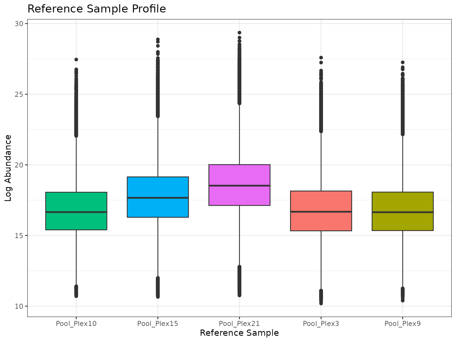
When we’re ready to actually perform the reference pool
normalization, we can do so as follows with the apply_norm
argument.
# Now apply the normalization; can use plot() to view the study samples after reference pool normalization
mypep <- normalize_isobaric(
  omicsData = mypep,
  exp_cname = "Plex",
  apply_norm = TRUE,
  refpool_cname = "Virus",
  refpool_notation = "Pool"
)
We can plot the samples after normalization to the reference pool.
plot(mypep)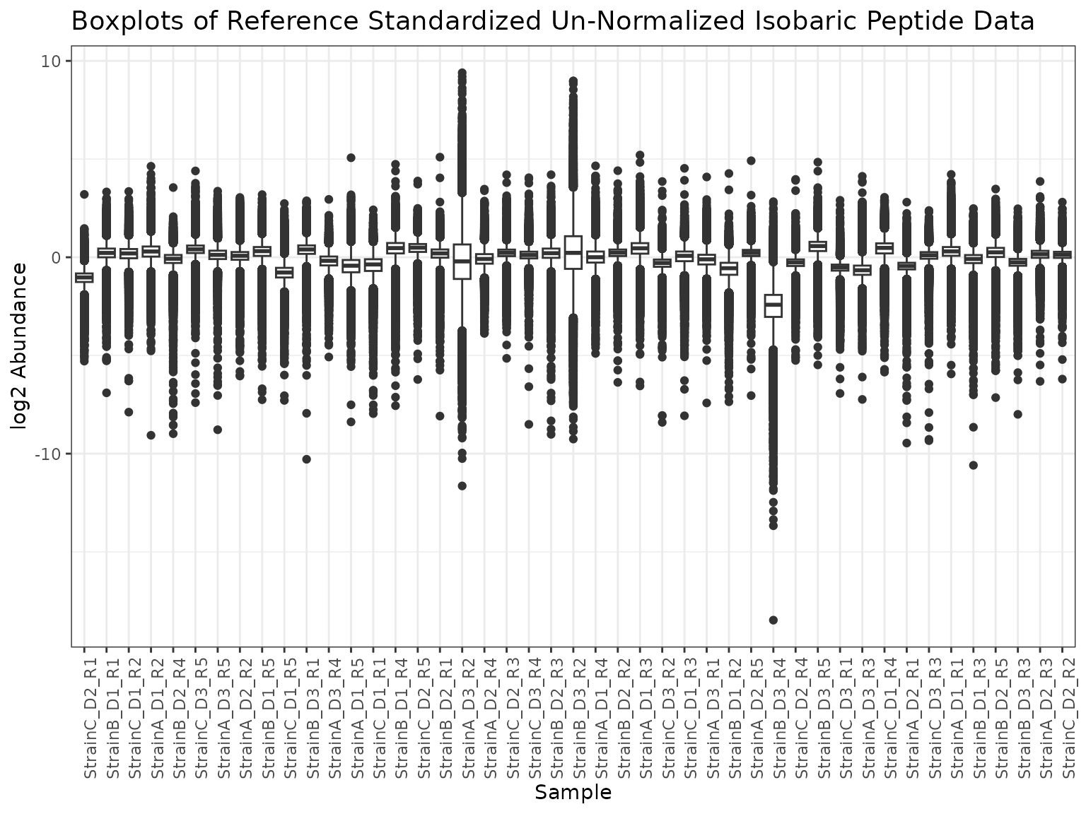
Workflow
Once the omicsData object is created, and after normalization to the reference pool samples for labeled peptide data, a typical QC workflow follows the figure below.
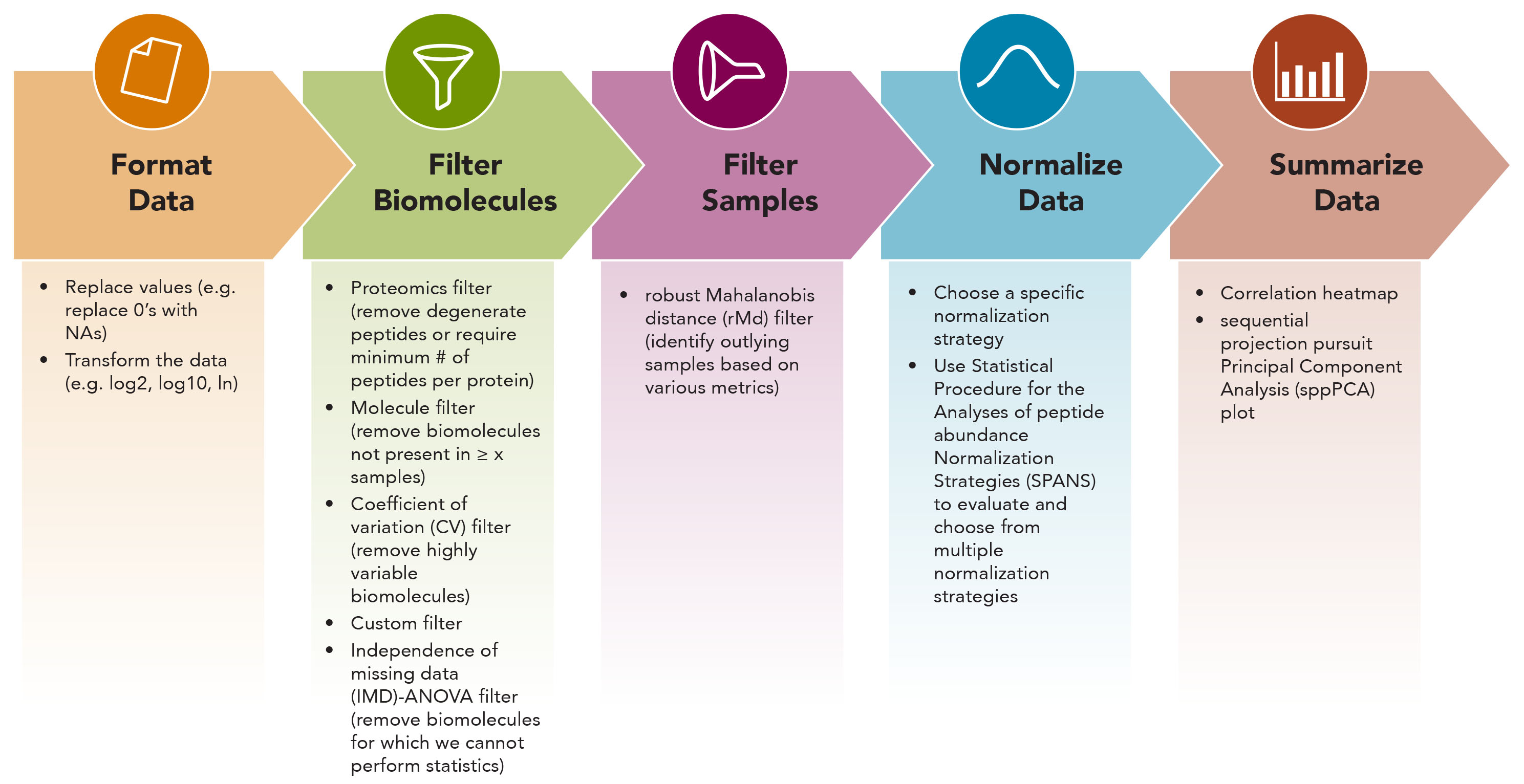
Figure 1. Quality control and processing workflow in pmartR package.
Main Effects
We are preparing this data for statistical analysis where we will
compare the samples belonging to one group to the samples belonging to
another, and so we must specify the group membership of the samples. We
do this using the group_designation() function, which
modifies our pepData object and returns an updated version of it. Up to
two main effects and up to two covariates may be specified, with one
main effect being required at minimum. For these example data, we
specify the main effect to be “Virus” so that we can make comparisons
between the different strains. Certain functions we will use below
require that groups have been designated via the
group_designation() function, and doing so makes the
results of plot and summary more
meaningful.
mypep <- group_designation(omicsData = mypep, main_effects = "Virus")
summary(mypep)
##
## Class isobaricpepData
## Unique SampleIDs (f_data) 45
## Unique Peptides (e_data) 215220
## Unique Proteins (e_meta) 16259
## Missing Observations 5541265
## Proportion Missing 0.572
## Samples per group: StrainC 15
## Samples per group: StrainB 15
## Samples per group: StrainA 15
plot(mypep, order_by = "Virus", color_by = "Virus")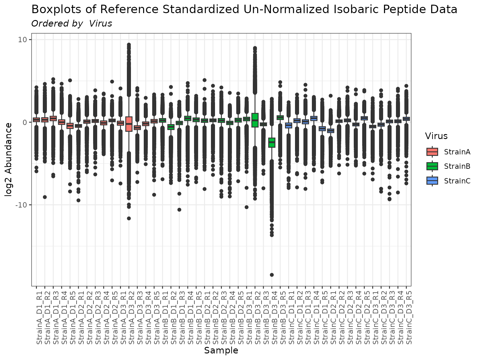
The group_designation() function creates an attribute of
the dataset as follows:
attributes(mypep)$group_DF## SampleID Group
## 1 StrainC_D2_R1 StrainC
## 2 StrainB_D1_R1 StrainB
## 3 StrainC_D1_R2 StrainC
## 4 StrainA_D1_R2 StrainA
## 5 StrainB_D2_R4 StrainB
## 6 StrainC_D3_R5 StrainC
## 7 StrainA_D3_R5 StrainA
## 8 StrainA_D2_R2 StrainA
## 9 StrainA_D3_R2 StrainA
## 10 StrainB_D1_R5 StrainB
## 11 StrainC_D1_R5 StrainC
## 12 StrainB_D3_R1 StrainB
## 13 StrainA_D3_R4 StrainA
## 14 StrainA_D1_R5 StrainA
## 15 StrainC_D1_R1 StrainC
## 16 StrainB_D1_R4 StrainB
## 17 StrainC_D2_R5 StrainC
## 18 StrainB_D2_R1 StrainB
## 19 StrainA_D2_R4 StrainA
## 20 StrainC_D2_R3 StrainC
## 21 StrainC_D3_R4 StrainC
## 22 StrainB_D2_R3 StrainB
## 23 StrainB_D3_R2 StrainB
## 24 StrainA_D1_R4 StrainA
## 25 StrainB_D2_R2 StrainB
## 26 StrainA_D1_R3 StrainA
## 27 StrainC_D3_R2 StrainC
## 28 StrainC_D1_R3 StrainC
## 29 StrainA_D3_R1 StrainA
## 30 StrainB_D1_R2 StrainB
## 31 StrainA_D2_R5 StrainA
## 32 StrainB_D3_R4 StrainB
## 33 StrainC_D2_R4 StrainC
## 34 StrainB_D3_R5 StrainB
## 35 StrainC_D3_R1 StrainC
## 36 StrainA_D3_R3 StrainA
## 37 StrainC_D1_R4 StrainC
## 38 StrainA_D2_R1 StrainA
## 39 StrainC_D3_R3 StrainC
## 40 StrainA_D1_R1 StrainA
## 41 StrainB_D1_R3 StrainB
## 42 StrainB_D2_R5 StrainB
## 43 StrainB_D3_R3 StrainB
## 44 StrainA_D2_R3 StrainA
## 45 StrainC_D2_R2 StrainCFilter Biomolecules
It is often good practice to filter out biomolecules that do not meet
certain criteria, and we offer up to 5 different filters to do this.
Each of the filter functions calculates metric(s) that can be used to
filter out biomolecules and returns an S3 object. Using the
summary() function produces a summary of the metric(s) and
using the plot() function produces a graph. Filters that
require a user-specified threshold in order to actually filter out
biomolecules have corresponding summary and
plot methods that take optional argument(s) to specify that
threshold. Once one of the filter functions has been called, the results
of that function can be used in conjunction with the
applyFilt() function to actually filter out peptides based
on the metric(s) and user-specified threshold(s) and create a new,
filtered omicsData object.
Proteomics Filter
The proteomics filter is applicable only to peptide level data
(isobaricpepData or pepData objects) that
contain the e_meta component, as this filter counts the
number of peptides that map to each protein and/or the number of
proteins to which each individual peptide maps.
Using the argument redundancy =
TRUE, we see from thesummary` that each peptide maps to a
single protein, so there are no redundant peptides to remove.
myfilter <- proteomics_filter(mypep)
summary(myfilter, redundancy = TRUE)
##
## Summary of Proteomics Filter
##
## Obs Proteins Per Peptide Obs Peptides Per Protein
## Min. 1 1
## 1st Qu. 1 1
## Median 1 5
## Mean 1 13.2369764438157
## 3rd Qu. 1 17
## Max. 1 639
##
## Peptides Proteins
## Filtered 0 0
## Not Filtered 215220 16259
plot(myfilter, bw_theme = TRUE)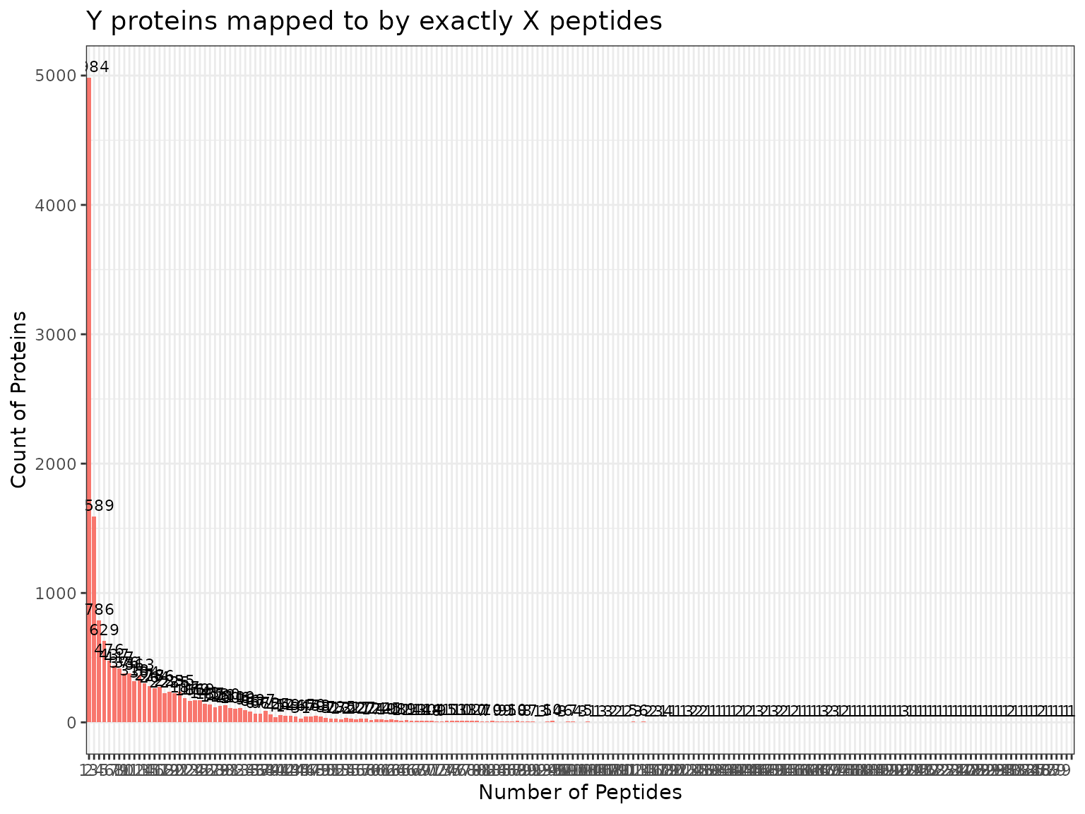
Using the argument min_num_peps, we can restrict our
dataset to just those proteins with a minimum number of peptides mapping
to them. A common threshold to use is 2, as this ensures that only
proteins with at least 2 peptides mapping to them are retained. We can
apply the proteomics filter using the applyFilt
function.
summary(myfilter, min_num_peps = 2)##
## Summary of Proteomics Filter
##
## Obs Proteins Per Peptide Obs Peptides Per Protein
## Min. 1 1
## 1st Qu. 1 1
## Median 1 5
## Mean 1 13.2369764438157
## 3rd Qu. 1 17
## Max. 1 639
##
## Peptides Proteins
## Filtered 4984 4984
## Not Filtered 210236 11275
# apply the filter, requiring proteins to have at least 2 peptides that map to them
mypep <- applyFilt(filter_object = myfilter, omicsData = mypep, min_num_peps = 2)
Molecule Filter
The molecule filter allows the user to remove from the dataset any
biomolecule not seen in at least min_num samples. The user
may specify a threshold of the minimum number of times each biomolecule
must be observed across all samples; the default value is 2. See the
“Filter Functionality” vignette for more detail about this filter, and
how to account for main effects and/or batches.
myfilter <- molecule_filter(mypep)
summary(myfilter, min_num = 3)
##
## Summary of Molecule Filter
## ----------------------------------
## Minimum Number:3
## Filtered:60349
## Not Filtered:149887
##
## num_observations frequency_counts
## 1 60340
## 2 60349
## 3 60361
## 4 60380
## 5 60405
## 6 60446
## 7 60505
## 8 60593
## 9 60822
## 10 66711
## 11 105829
## 12 105844
## 13 105855
## 14 105865
## 15 105890
## 16 105922
## 17 105957
## 18 106022
## 19 106120
## 20 106345
## 21 111160
## 22 135001
## 23 136474
## 24 136480
## 25 136495
## 26 136518
## 27 136549
## 28 136589
## 29 136636
## 30 136742
## 31 136966
## 32 139884
## 33 159015
## 34 165736
## 35 165750
## 36 165758
## 37 165765
## 38 165785
## 39 165804
## 40 165833
## 41 165910
## 42 166014
## 43 166299
## 44 172725
## 45 210236
plot(myfilter, bw_them = TRUE)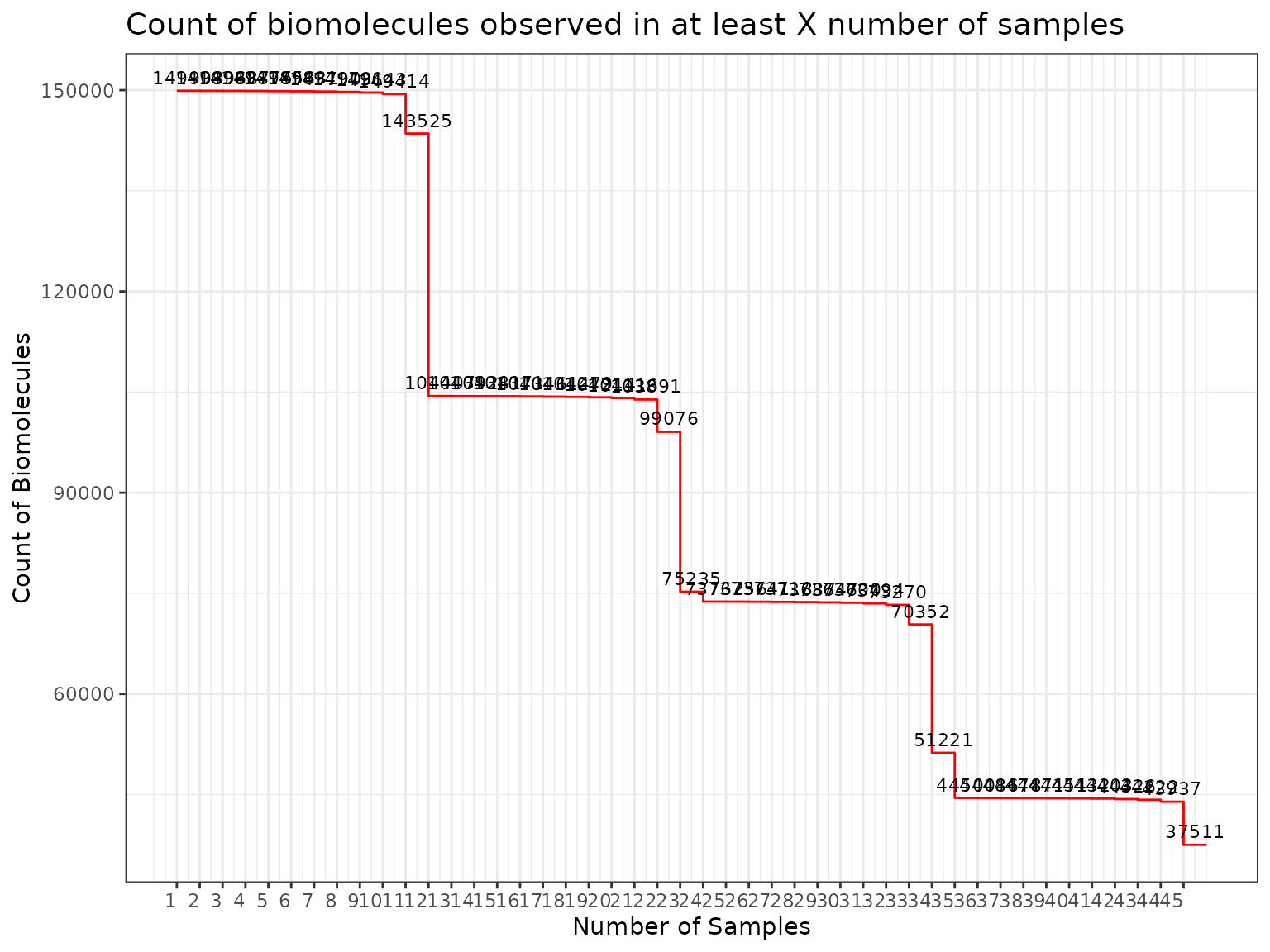
Setting the threshold to 3, we would filter 60,349 peptides out of
the dataset. If we’d like to make the filter less stringent, we could
use a threshold of 2. We use the applyFilt function to
apply the molecule filter.
summary(myfilter, min_num = 2)##
## Summary of Molecule Filter
## ----------------------------------
## Minimum Number:2
## Filtered:60340
## Not Filtered:149896
##
## num_observations frequency_counts
## 1 60340
## 2 60349
## 3 60361
## 4 60380
## 5 60405
## 6 60446
## 7 60505
## 8 60593
## 9 60822
## 10 66711
## 11 105829
## 12 105844
## 13 105855
## 14 105865
## 15 105890
## 16 105922
## 17 105957
## 18 106022
## 19 106120
## 20 106345
## 21 111160
## 22 135001
## 23 136474
## 24 136480
## 25 136495
## 26 136518
## 27 136549
## 28 136589
## 29 136636
## 30 136742
## 31 136966
## 32 139884
## 33 159015
## 34 165736
## 35 165750
## 36 165758
## 37 165765
## 38 165785
## 39 165804
## 40 165833
## 41 165910
## 42 166014
## 43 166299
## 44 172725
## 45 210236##
## Class isobaricpepData
## Unique SampleIDs (f_data) 45
## Unique Peptides (e_data) 149896
## Unique Proteins (e_meta) 10220
## Missing Observations 2621489
## Proportion Missing 0.389
## Samples per group: StrainC 15
## Samples per group: StrainB 15
## Samples per group: StrainA 15Coefficient of Variation Filter
The coefficient of variation (CV) filter calculates the pooled CV values as in (Ahmed 1995).
The user can then specify a CV threshold, above which peptides are removed.
##
## Summary of Coefficient of Variation (CV)
## Filter
## ----------------------
## CVs:
##
##    Min. 1st Qu.  Median    Mean 3rd Qu.    Max.
##   1.231  30.605  35.206  38.178  41.904 246.023
##
## Total NAs: 7
## Total Non-NAs: 149889
##
## Number Filtered Biomolecules: 146
plot(myfilter, cv_threshold = 140)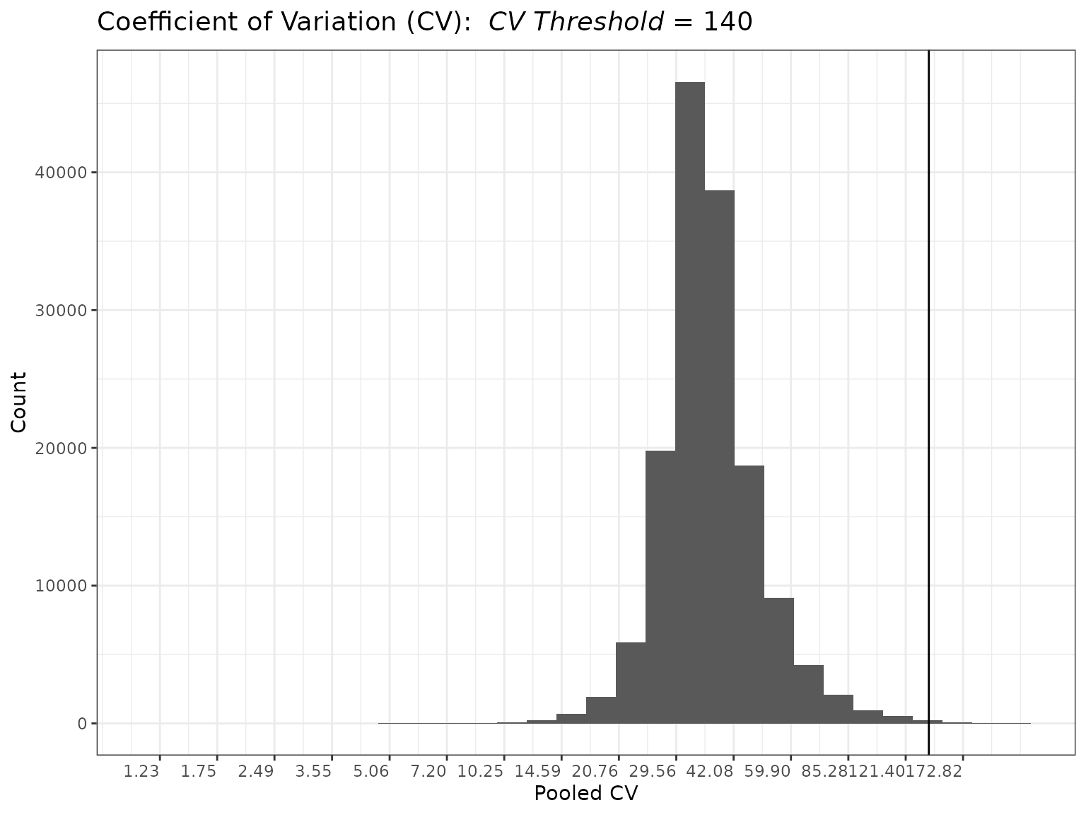
##
## Class                      isobaricpepData
## Unique SampleIDs (f_data)               45
## Unique Peptides (e_data)            149750
## Unique Proteins (e_meta)             10220
## Missing Observations               2620981
## Proportion Missing                   0.389
## Samples per group: StrainC              15
## Samples per group: StrainB              15
## Samples per group: StrainA              15
Custom Filter
Sometimes it is known a priori that certain peptides or samples should be filtered out of the dataset prior to statistical analysis. Perhaps there are known contaminant proteins, and so peptides mapping to them should be removed, or perhaps something went wrong during sample preparation for a particular sample. On the other hand, it may be preferred to specify peptides or samples to keep (removing those not explicitly specified), and this can also be accomplished. Keep in mind that both ‘remove’ and ‘keep’ arguments cannot be specified together; either ‘remove’ arguments only or ‘keep’ arguments only may be specified in a single call to custom_filter().
Here, we demonstrate the removal of contaminant proteins and their associated peptides; the contaminant protein names contain “XXX”.
remove_prots <- mypep$e_meta$Protein[grep("XXX", mypep$e_meta$Protein)]
myfilter <- custom_filter(mypep, e_meta_remove = remove_prots)
summary(myfilter)
##
## Summary of Custom Filter
##
## Filtered Remaining Total
## SampleIDs (f_data) 0 45 45
## Peptides (e_data) 481 149269 149750
## Proteins (e_meta) 481 9739 10220
mypep <- applyFilt(filter_object = myfilter, omicsData = mypep)Note that there is a summary() method for objects of
type custom_filt, but no plot() method.
IMD-ANOVA Filter
The IMD-ANOVA filter removes biomolecules that do not have sufficient
data for the statistical tests available in pmartR; these
are ANOVA (quantitative test) and an independence of missing data (IMD)
using a g-test (qualitative test). When using the
summary(), plot(), and
applyFilt() functions, you can specify just one filter
(ANOVA or IMD) or both, depending on the tests you’d like to perform
later.
First we create the filter object.
myfilter <- imdanova_filter(mypep)Here we consider what the filter would look like for both ANOVA and IMD.
summary(myfilter, min_nonmiss_anova = 2, min_nonmiss_gtest = 3)##
## Summary of IMD-ANOVA Filter
##
## Total Observations: 149269
## Filtered: 26
## Not Filtered: 149243Here we consider what the filter would look like for just ANOVA.
summary(myfilter, min_nonmiss_anova = 2)##
## Summary of IMD-ANOVA Filter
##
## Total Observations: 149269
## Filtered: 41
## Not Filtered: 149228Here we consider what the filter would look like for just IMD.
summary(myfilter, min_nonmiss_gtest = 3)##
## Summary of IMD-ANOVA Filter
##
## Total Observations: 149269
## Filtered: 49
## Not Filtered: 149220Now we apply the filter for both ANOVA and IMD.
mypep <- applyFilt(filter_object = myfilter, omicsData = mypep, min_nonmiss_anova = 2, min_nonmiss_gtest = 3)## You have specified remove_singleton_groups = TRUE, but there are no singleton groups to remove. Proceeding with application of the IMD-ANOVA filter.
summary(mypep)##
## Class isobaricpepData
## Unique SampleIDs (f_data) 45
## Unique Peptides (e_data) 149243
## Unique Proteins (e_meta) 9830
## Missing Observations 2604500
## Proportion Missing 0.388
## Samples per group: StrainC 15
## Samples per group: StrainB 15
## Samples per group: StrainA 15Filter Samples
To identify any samples that are potential outliers or anomalies (due to sample quality, preparation, or processing circumstances), we use a robust Mahalanobis distance (rMd) (Matzke et al. 2011) score based on 2-5 metrics. The possible metrics are:
Correlation
Proportion of data that is missing (“Proportion_Missing”)
Median absolute deviation (“MAD”)
Skewness
Kurtosis
The rMd score can be mapped to a p-value, and a p-value threshold used to identify potentially outlying samples. In general, for proteomics data we recommend using all 5 metrics (or sometimes leaving out Kurtosis). A plot of the rMd values for each sample is generated, and specifying a value for ‘pvalue_threshold’ results in a horizontal line on the plot, with samples above the line slated for filtering at the given threshold.
myfilter <- rmd_filter(omicsData = mypep, metrics = c("Correlation", "Proportion_Missing", "MAD", "Skewness"))
plot(myfilter)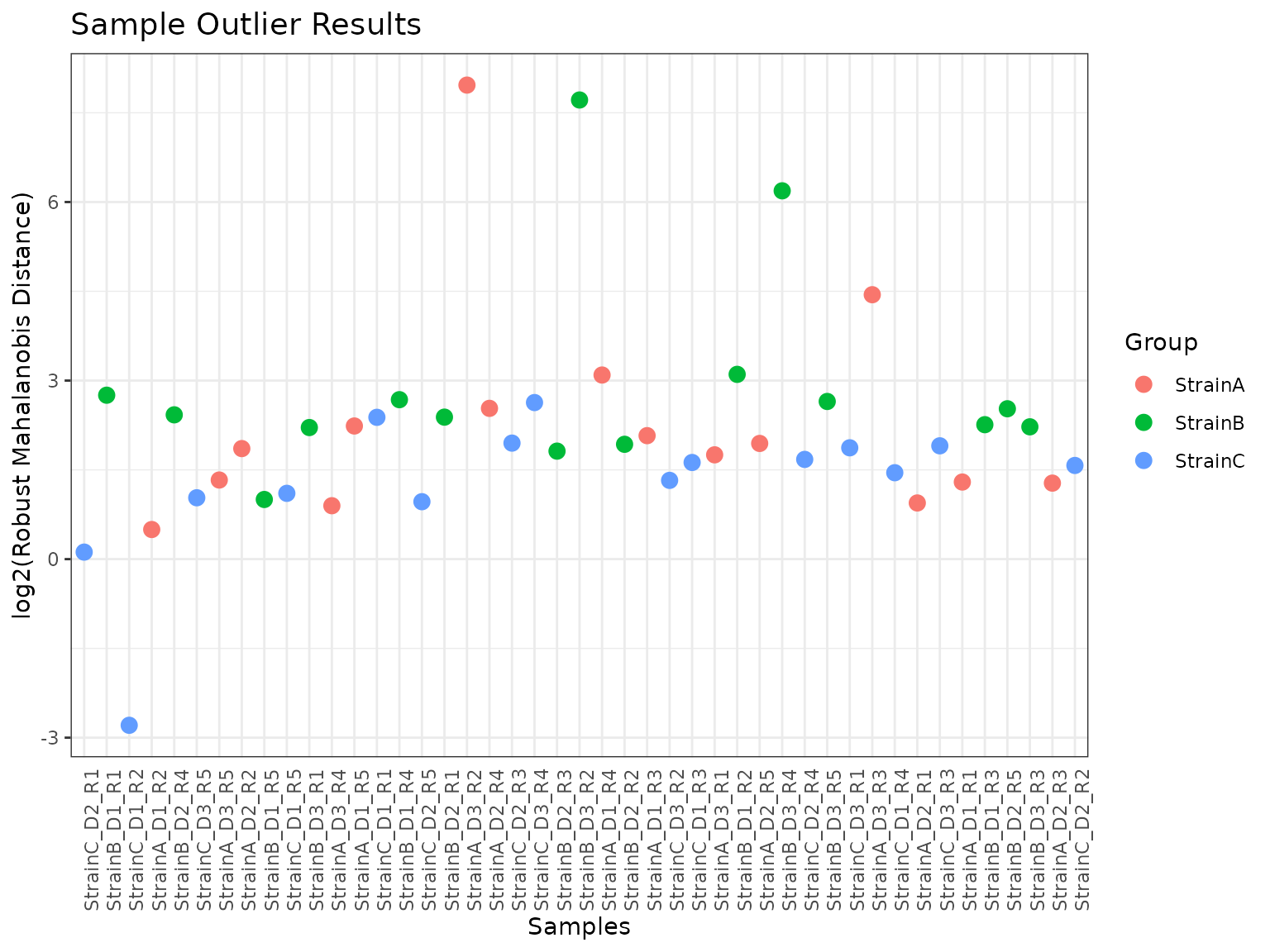
summary(myfilter, pvalue_threshold = 0.0001)##
## Summary of RMD Filter
## ----------------------
## P-values:
##
## Min. 1st Qu. Median Mean 3rd Qu. Max.
## 0.0000 0.2177 0.4325 0.4292 0.6442 0.9975
##
## Metrics Used: MAD, Skewness, Corr, Proportion_Missing
##
## Filtered Samples: StrainA_D3_R2, StrainB_D3_R2, StrainB_D3_R4
plot(myfilter, pvalue_threshold = 0.0001, bw_theme = TRUE)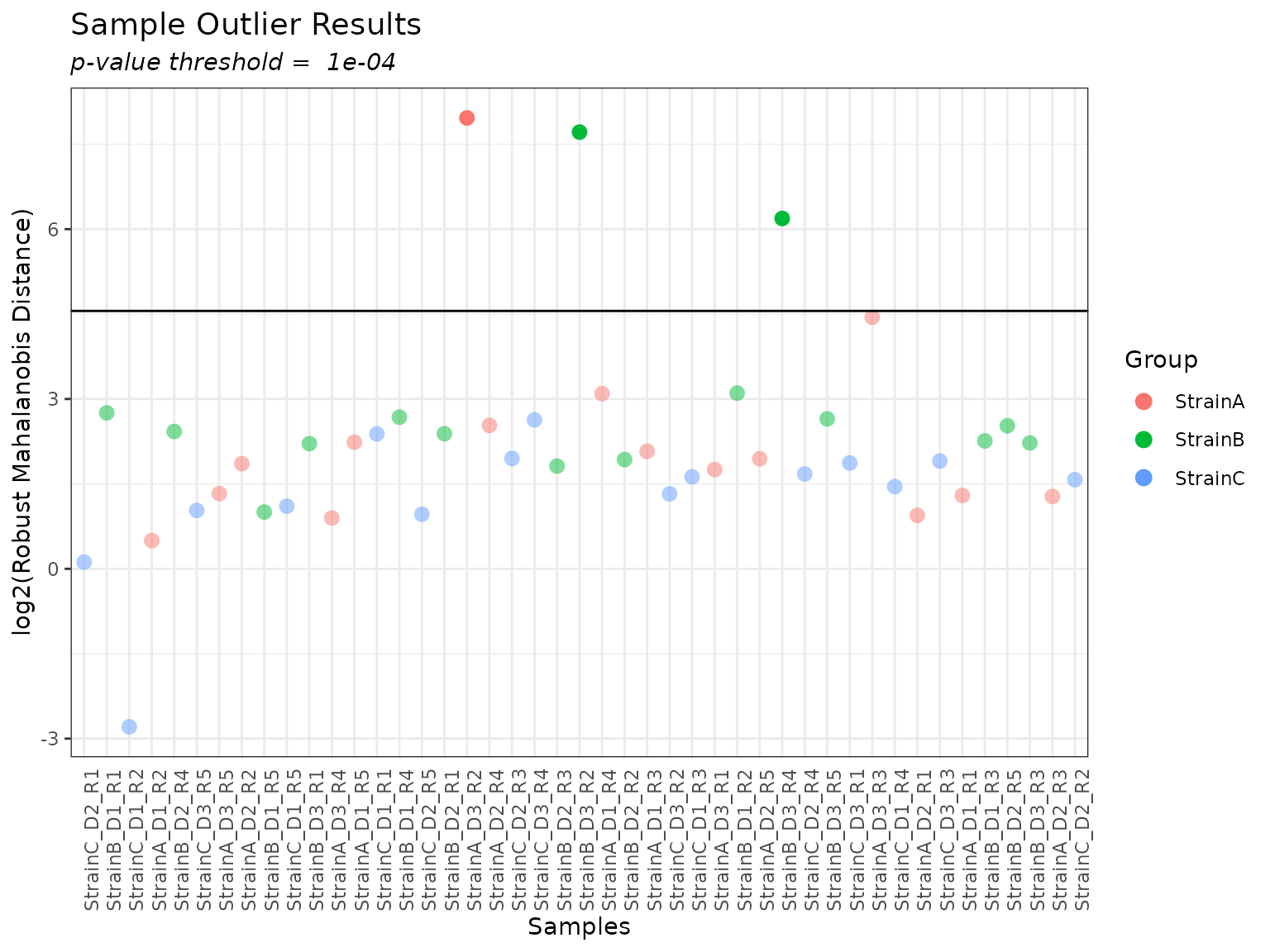
Using the output from the summary() function, we can
explore the potential outliers identified to see which metrics are
driving their “outlier-ness”. Box plots for each metric are graphed,
with the specified sample marked with an X.
# get vector of potential outliers
potential_outliers <- summary(myfilter, pvalue_threshold = 0.0001)$filtered_samples

# loop over potential outliers to generate plots
if (length(potential_outliers) > 0) {
  for (i in 1:length(potential_outliers)) {
    print(plot(myfilter, sampleID = potential_outliers[i]))
  }
}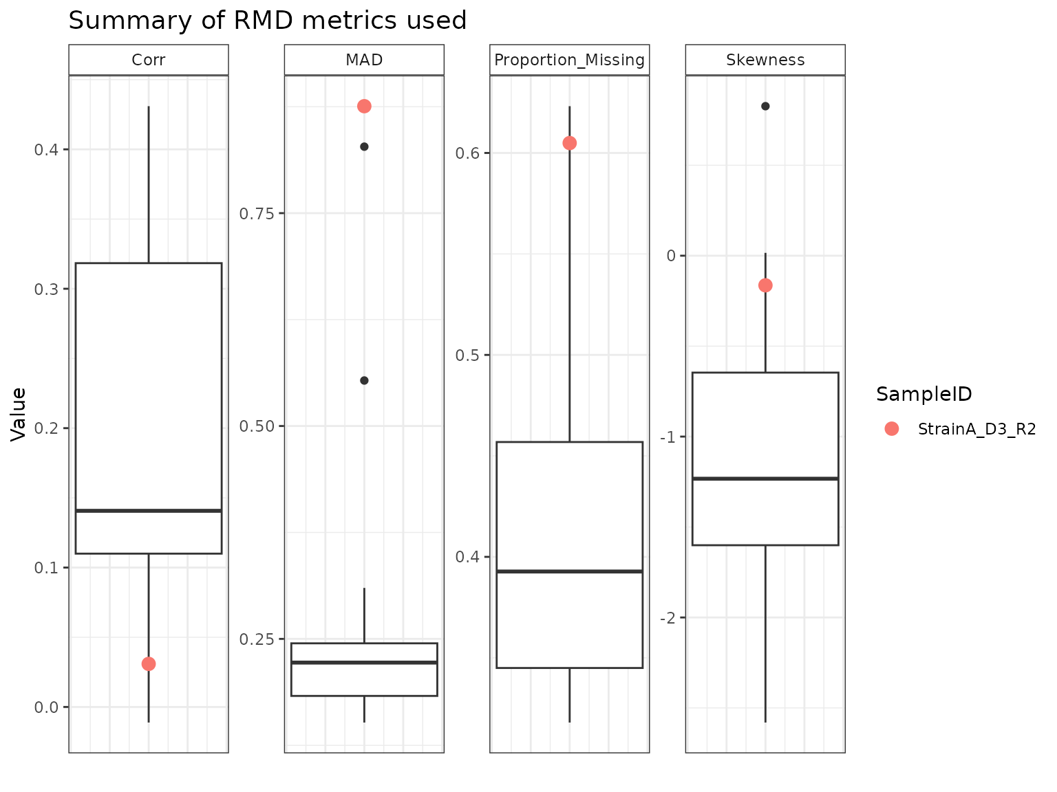
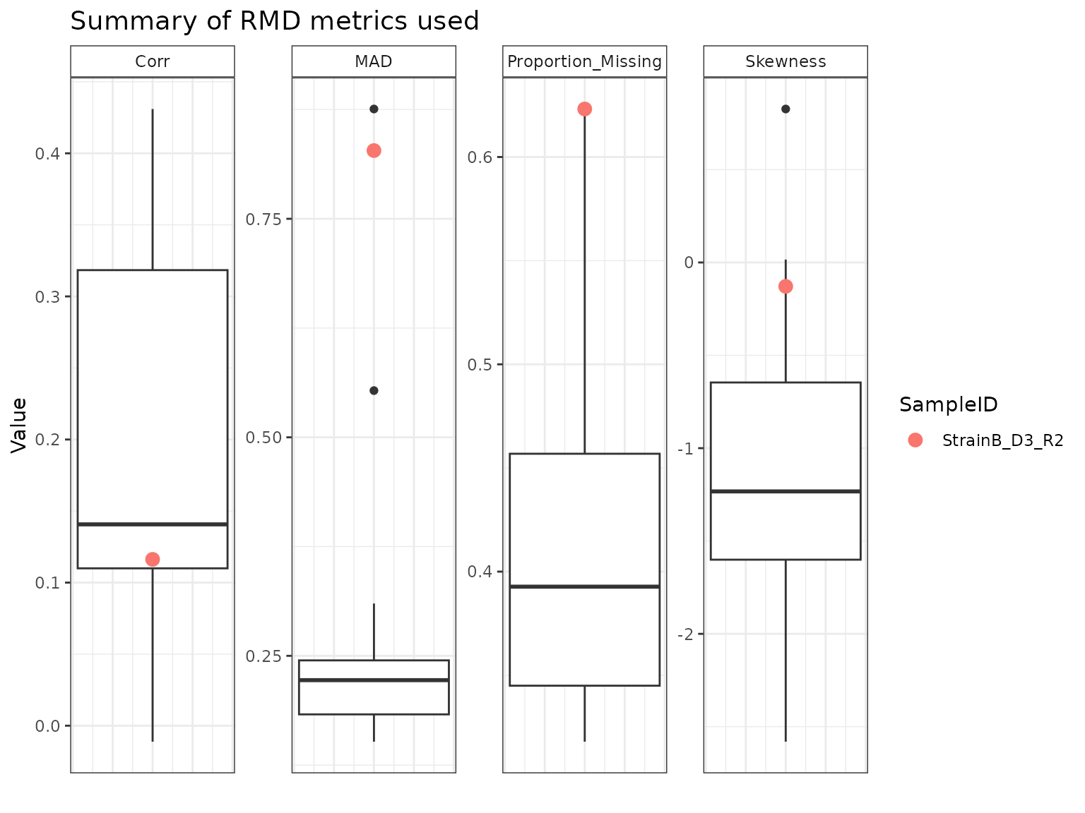
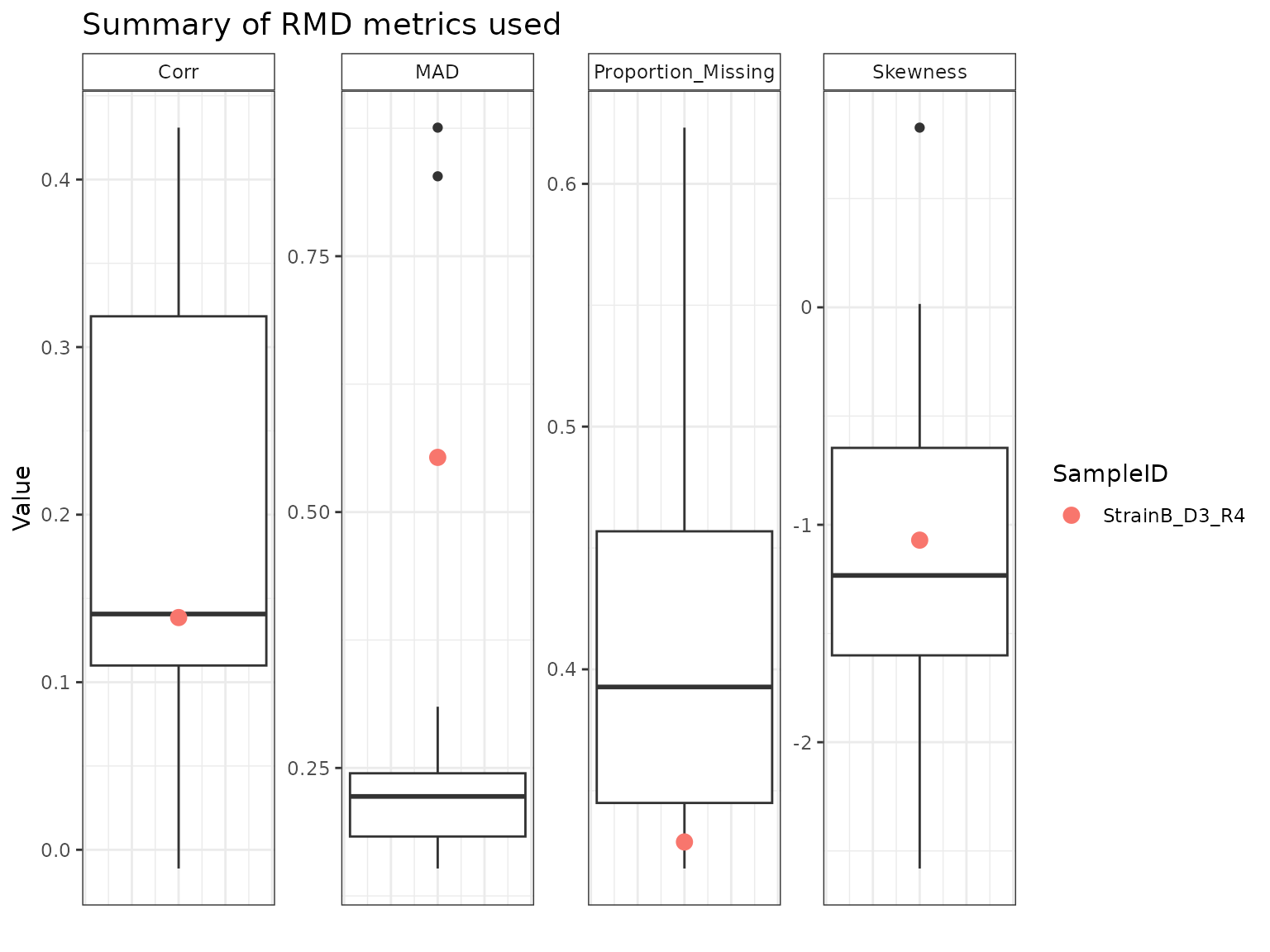
StrainB_D3_R4 appears to have been flagged as a potential outlier primarily on the basis of its MAD relative to the other samples. StrainA_D3_R2 and StrainB_D3_R2 have similar profiles across the four metrics, with high amounts of missing data, low correlations, and high MAD and skew.
We can use this information to help determine whether to remove any of these samples. It is often useful to look at additional data summaries to inform outlier removal, such as a correlation heat map or principal components analysis (PCA) plot.
In the correlation heatmap we are looking to see if any samples stand
out as having low correlation with a majority of the others; any such
samples would appear as dark stripes. We use the
interactive = TRUE argument so we can hover over the plot
and see which samples correspond to the cells in the heatmap. None of
the samples stands out as concerning in the correlation heatmap for
these data.
mycor <- cor_result(omicsData = mypep)
plot(mycor, interactive = TRUE)
The PCA function in pmartR utilizes (Stacklies et al. 2007) probabilistic PCA, which
which allows for missing data. In the PCA plot we are interested to see
whether any of the potential outliers identified by the rMd filter do
not cluster with their main effect group. Note that for large proteomics
datasets, such as this example, generating the PCA results may take up
to a minute or longer.
Using the interactive = TRUE argument to the plot
function, we can see that the three potential outliers identified by the
rMd filter are the same samples that do not cluster with the others
(paying attention to the R^2 values on the axes).
Randomness is present in probabilistic PCA computations, set.seed() can be used to ensure consistent results.
set.seed(2025)

mypca <- dim_reduction(omicsData = mypep)

plot(mypca, interactive = TRUE)
Given the above exploratory analyses, we’d recommend removing all three samples identified by the rMd filter. Note that if we had only wanted to remove a subset of those samples, we could do so with a custom filter, as opposed to applying the rMd filter.
mypep <- applyFilt(filter_object = myfilter, omicsData = mypep, pvalue_threshold = 0.0001)
summary(mypep)
##
## Class isobaricpepData
## Unique SampleIDs (f_data) 42
## Unique Peptides (e_data) 149243
## Unique Proteins (e_meta) 9830
## Missing Observations 2372136
## Proportion Missing 0.378
## Samples per group: StrainC 15
## Samples per group: StrainB 13
## Samples per group: StrainA 14Summarize Data
In addition to the correlation heatmap and PCA plot that we utilized
above, the pmartR package contains additional methods for
data summarization and exploration that can be used as part of the QC
process: numeric summaries and associated plots (via the
edata_summary function), missing data summarization (via
missingval_result, plot_missingval,
missingval_scatterplot and
missingval_heatmap).
Numeric Summaries
We can generate numeric summaries of our data by either sample or
molecule. The edata_summary function computes the mean,
standard deviation, median, percent of observations for which a value
was observed, the minimum value, and the maximum value.
edata_summary(mypep, by = "sample", groupvar = NULL)## mean
## sample mean
## 1 StrainC_D2_R1 -1.06143305348409
## 2 StrainB_D1_R1 0.20536249801376
## 3 StrainC_D1_R2 0.158855539253571
## 4 StrainA_D1_R2 0.280642605803086
## 5 StrainB_D2_R4 -0.115955261298007
## 6 ---- ----
## 38 StrainB_D1_R3 -0.112316793848367
## 39 StrainB_D2_R5 0.23073893517671
## 40 StrainB_D3_R3 -0.278105412627509
## 41 StrainA_D2_R3 0.121439492777355
## 42 StrainC_D2_R2 0.0971310640249695
##
## std_dev
## sample sd
## 1 StrainC_D2_R1 0.410541305359474
## 2 StrainB_D1_R1 0.447659771270713
## 3 StrainC_D1_R2 0.461345839153307
## 4 StrainA_D1_R2 0.461551494959209
## 5 StrainB_D2_R4 0.420592822397728
## 6 ---- ----
## 38 StrainB_D1_R3 0.427848475258554
## 39 StrainB_D2_R5 0.44500111374766
## 40 StrainB_D3_R3 0.368193551096942
## 41 StrainA_D2_R3 0.402055500910083
## 42 StrainC_D2_R2 0.330191038717702
##
## median
## sample median
## 1 StrainC_D2_R1 -1.027005550312
## 2 StrainB_D1_R1 0.222200216723788
## 3 StrainC_D1_R2 0.196373098918481
## 4 StrainA_D1_R2 0.295098732824351
## 5 StrainB_D2_R4 -0.0753256791351191
## 6 ---- ----
## 38 StrainB_D1_R3 -0.0872785367349405
## 39 StrainB_D2_R5 0.251012917359553
## 40 StrainB_D3_R3 -0.256438764618135
## 41 StrainA_D2_R3 0.155072201518131
## 42 StrainC_D2_R2 0.133396561245203
##
## pct_obs
## sample pct_obs
## 1 StrainC_D2_R1 0.597924190749315
## 2 StrainB_D1_R1 0.60626629054629
## 3 StrainC_D1_R2 0.606715222824521
## 4 StrainA_D1_R2 0.606768826678638
## 5 StrainB_D2_R4 0.606018372720999
## 6 ---- ----
## 38 StrainB_D1_R3 0.654730875149923
## 39 StrainB_D2_R5 0.654965392011686
## 40 StrainB_D3_R3 0.654710773704629
## 41 StrainA_D2_R3 0.655032396829332
## 42 StrainC_D2_R2 0.65498549345698
##
## minimum
## sample min
## 1 StrainC_D2_R1 -5.28803117525946
## 2 StrainB_D1_R1 -6.90296758852084
## 3 StrainC_D1_R2 -7.88599163997331
## 4 StrainA_D1_R2 -9.0641588168261
## 5 StrainB_D2_R4 -8.98433240365627
## 6 ---- ----
## 38 StrainB_D1_R3 -10.5926699621308
## 39 StrainB_D2_R5 -7.14495131542973
## 40 StrainB_D3_R3 -7.99796318332263
## 41 StrainA_D2_R3 -6.31873411525732
## 42 StrainC_D2_R2 -6.2030259000209
##
## maximum
## sample max
## 1 StrainC_D2_R1 3.20201396788793
## 2 StrainB_D1_R1 3.32745017274159
## 3 StrainC_D1_R2 3.35107088869222
## 4 StrainA_D1_R2 4.63459394111101
## 5 StrainB_D2_R4 3.55081326856828
## 6 ---- ----
## 38 StrainB_D1_R3 2.48031626920593
## 39 StrainB_D2_R5 3.47439261166162
## 40 StrainB_D3_R3 2.47089345654322
## 41 StrainA_D2_R3 3.86159378287714
## 42 StrainC_D2_R2 2.47463437858901
# edata_summary(norm_data, by = "molecule", groupvar = "Condition")
# edata_summary(norm_data, by = "molecule", groupvar = NULL)
Missing Data
Patterns of missing data can be explored using the
missingval_result and plot_missingval
functions.
results <- missingval_result(omicsData = mypep)

plot(results, omicsData = mypep, plot_type = "bar")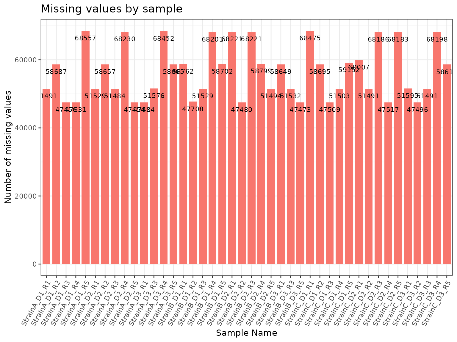
plot(results, omicsData = mypep, plot_type = "scatter")## Ignoring unknown labels:
## • colour : "Group"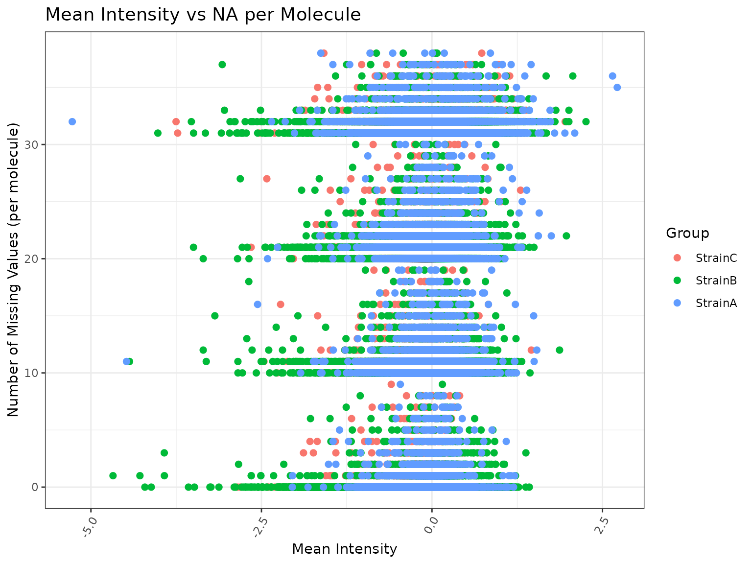
Normalize Data
After quality control, filtering, and exploring our data, the next
step in a typical workflow is to normalize the data. See the “Data
Normalization” vignette for more details about the normalization
approaches included in pmartR.
Since we are working with a global proteomics dataset, we will use the SPANS algorithm to guide our selection of normalization approach and then normalize the data. Datasets with only a couple hundred biomolecules or fewer are not candidates for SPANS. Note that running SPANS can take up to a couple of minutes or more.
# returns a data frame arranged by descending SPANS score
# not run due to long runtime; SPANS plot generated and saved to include in vignette
spans_result <- spans_procedure(mypep)

plot(spans_result)
Plotting the SPANS object returns a heatmap where each cell in the grid corresponds to one combination of subset and normalization function. A dot in the cell indicates that the method had the highest SPANS scores; ties are possible as we see below.
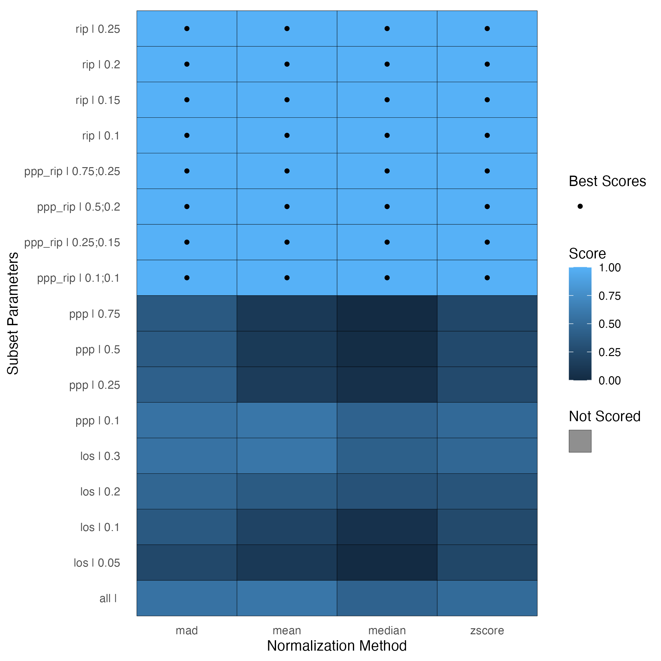
Particularly when there are ties in the SPANS scores, it can be
useful to see how many biomolecules are part of the subset(s) being
used. Basing a normalization on too few biomolecules, say fewer than
10%, is not advised. The column in the SPANSRes object
called “mols_used_in_norm” provides the number of biomolecules in the
subset. In our case, the subset RIP (0.25) contains 20753 peptides, so
we will select this subset. Since all normalization functions resulted
in the same SPANS score for this subset, we will choose median.
Similar to normalizing to the reference pool, we will first create a normRes object so we can see the effect of applying the specified normalization ahead of actually applying it to our data.
# readRDS("/vignettes/spans_result.RDS")

mynorm <- normalize_global(
  omicsData = mypep,
  subset_fn = "rip", params = list(rip = 0.25),
  norm_fn = "median",
  apply_norm = FALSE
)

# plot(mynorm) # currently errors out
Now that we are satisfied with our selections, we can apply the normalization
# apply the normalization
mynorm <- normalize_global(omicsData = mypep,
                           subset_fn = "rip", params = list(rip = 0.25),
                           norm_fn = "median",
                           apply_norm = TRUE)
At this point it may be of interest to re-evaluate some of the earlier exploratory analyses or plots.
Protein Quantification Methods
Protein quantification can be done using the
protein_quant function, either with or without accounting
for different isoforms of the proteins, which are also called
‘proteoforms’. Regardless of whether the user is accounting for protein
isoforms, they must specify a method for rolling peptides up to proteins
(one of “rollup”, “rollup”, “qrollup”, or “zrollup”) and a function to
use for combining the peptide-level data (either “mean” or “median”).
When the user does wish to account for protein isoforms, they may
utilize Bayesian Proteoform Quantification (BP-Quant) (Webb-Robertson et al. 2014) via the
bpquant function, and input those results as one of the
arguments to the protein_quant function.
The protein_quant function takes in an object of class
pepData (or isobaricpepData) and returns an
object of class proData.
Rollup Methods
The rollup method takes either the mean or median of all peptides mapping to a given protein, and sets that value as the relative protein abundance.
In the rrollup method, all peptides that map to a single protein are scaled based on a chosen reference peptide, which is the peptide with most observations. Next the average or mean of the scaled peptides is set as the relative protein abundance. (Matzke et al. 2013)
The qrollup method starts with all peptides that map to a single protein. Next peptides are chosen according to an abundance cutoff value and the average or mean of the scaled peptides is set as the protein abundance.
In the zrollup method, scaling is done similarly to the z-score formula (except with medians instead of means). The scaling formula is applied to peptides that map to a single protein and then the mean or median of the scaled peptides is set as protein abundance (from DAnTE article). The rollup method is similar to rrollup method, except there is no scaling involved in these methods. Either the mean or median is applied to all peptides that map to a single protein to obtain protein abundance. (Polpitiya et al. 2008)
Here we utilize rrollup.
mypro <- protein_quant(
  pepData = mypep,
  method = "rrollup",
  combine_fn = "median"
)

plot(mypro, order_by = "Virus", color_by = "Virus")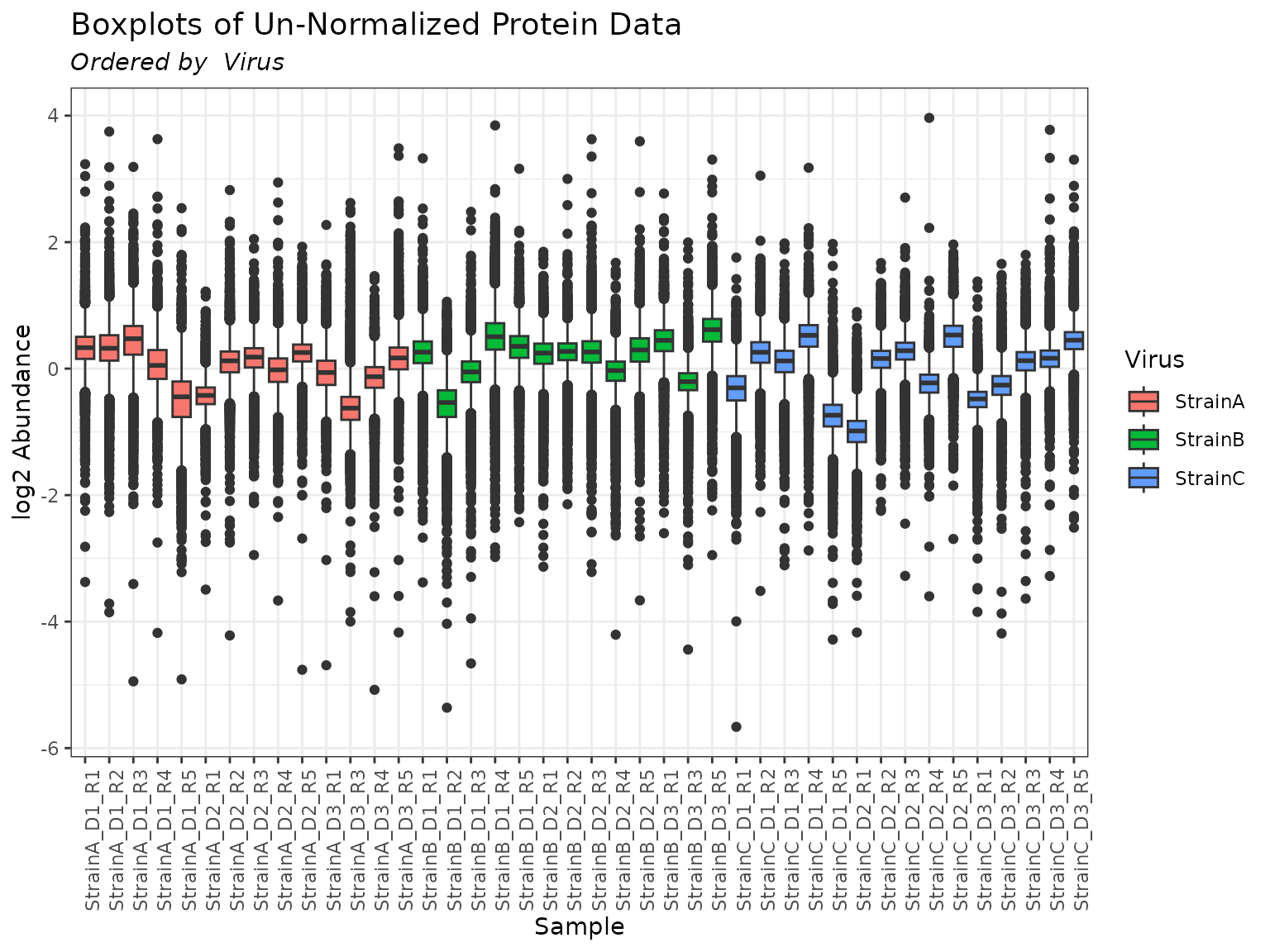
Statistical Comparisons
Now that we have data at the protein level, we will perform the
comparisons of interest for these data, namely all pairwise comparisons
between the virus strains. Note that this dataset is included in the
pmartRdata package and used as an example only. Information
about Donor’s is included for exemplar usage of a second main effect, if
desired. A valid statistical analysis for an experiment that involved
Donor’s or other units of repeated measurements cannot be performed
within pmartR. To account for random or mixed effects,
please consult with a statistician as needed. We commonly use the
lme4 library for this type of statistical analysis (Bates et al. 2015).
To make all pairwise comparisons between our 3 virus strains using
both ANOVA and the IMD-test (or g-test), we can use the
imd_anova function in the following way using defaults (no
p-value adjustments being the most important default to note). The
summary function provides an overview of the results of
these tests.
mystats <- imd_anova(omicsData = mypro, test_method = "combined")## Joining with `by = join_by(SampleID)`
## Joining with `by = join_by(Protein)`
summary(mystats)## Type of test: combined
##
## Multiple comparison adjustment ANOVA:
##
## Multiple comparison adjustment G-test:
##
## p-value threshold: 0.05
##
## Number of significant biomolecules by comparison. Columns specify fold change direction and type of test:
##
## Comparison Total:Positive Total:Negative Positive:ANOVA
## 1 StrainC_vs_StrainB 126 1999 126
## 2 StrainC_vs_StrainA 39 207 38
## 3 StrainB_vs_StrainA 1692 297 1691
## Negative:ANOVA Positive:G-test Negative:G-test
## 1 1999 0 0
## 2 206 1 1
## 3 296 1 1We can also use plot to obtain graphical results.
plot(mystats, plot_type = "volcano")## Joining with `by = join_by(Protein, Comparison)`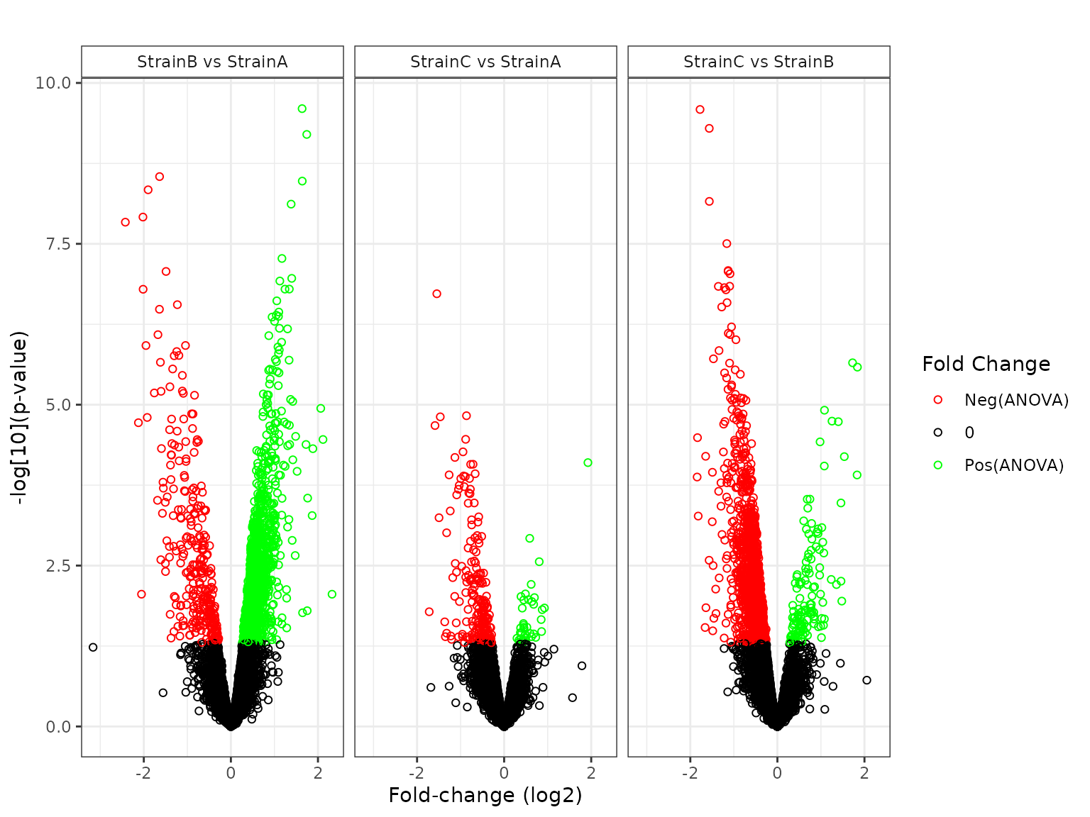
plot(mystats, plot_type = "bar")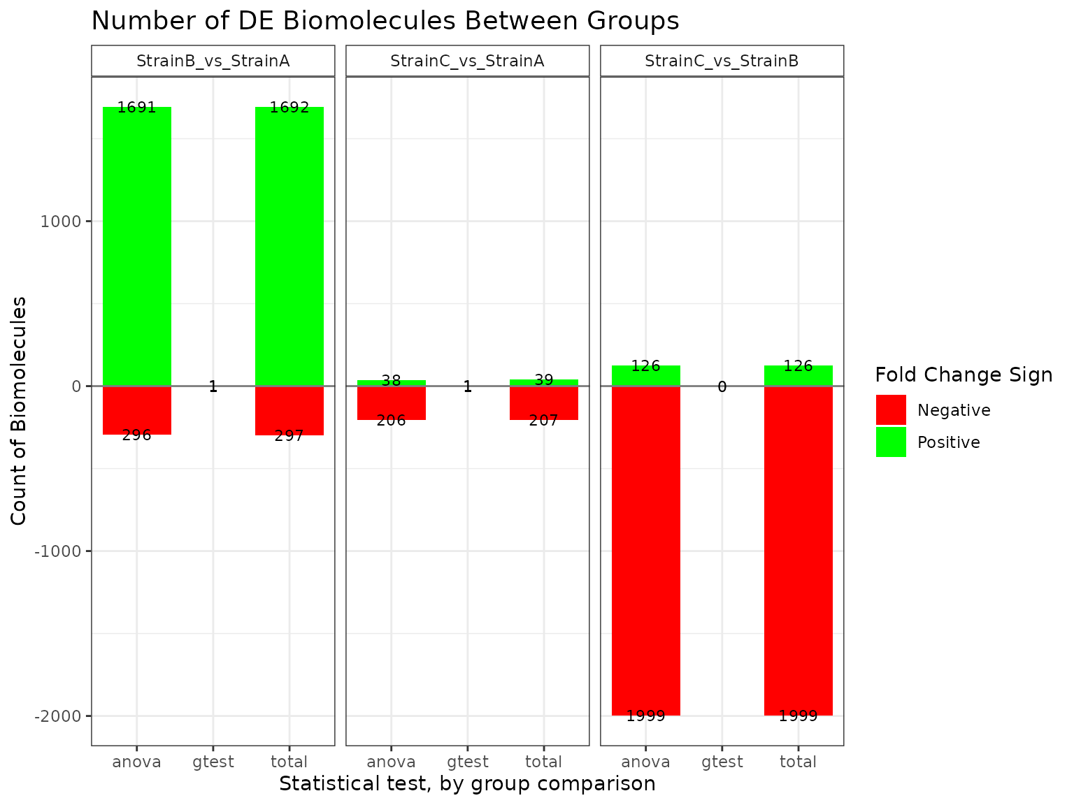
plot(mystats, plot_type = "gheatmap") # exclude this one?## Joining with `by = join_by(Protein, Comparison)`
## Joining with `by = join_by(Count_First_Group, Count_Second_Group, Comparison)`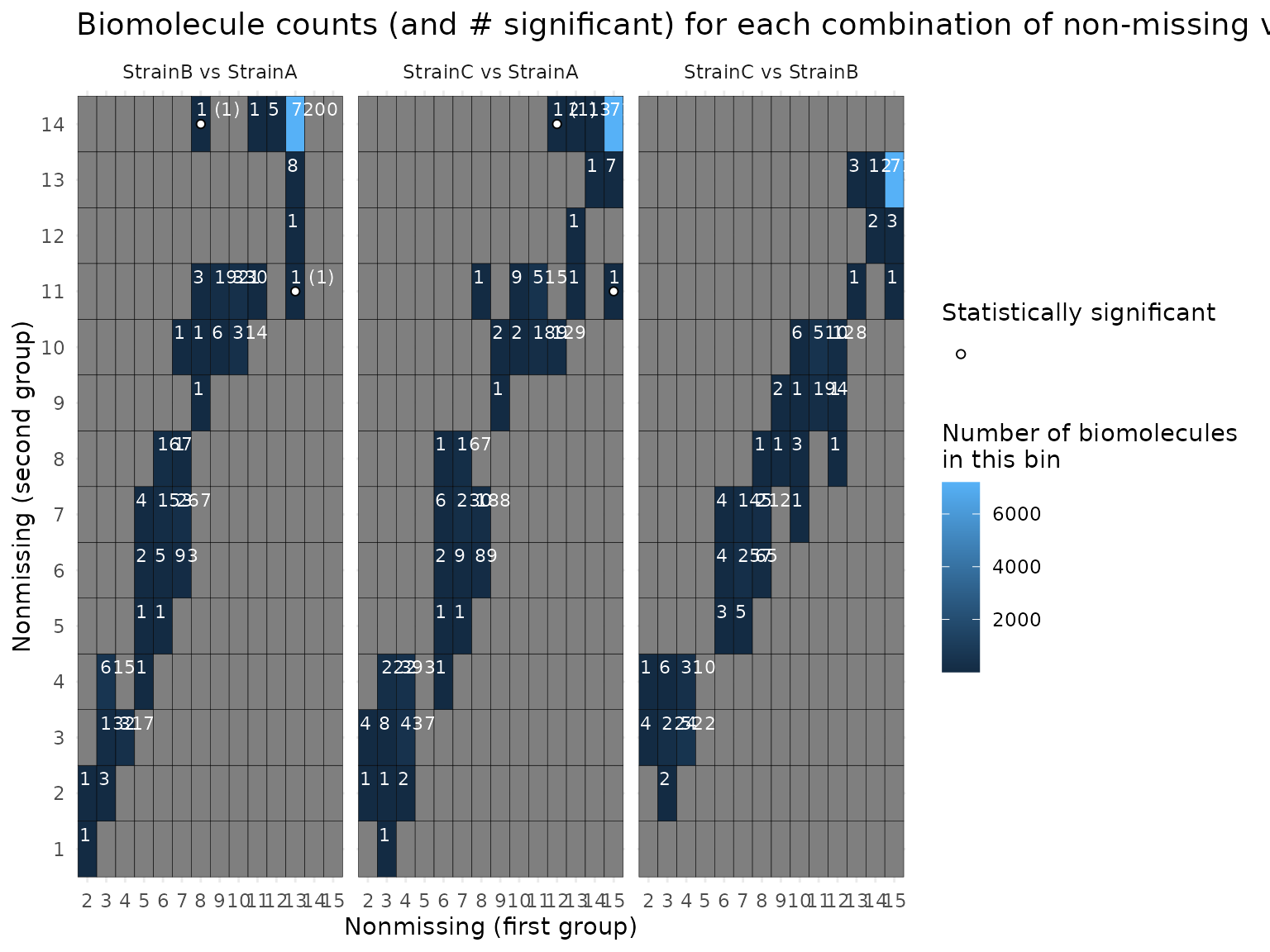
plot(mystats, plot_type = "fcheatmap")## Joining with `by = join_by(Protein, Comparison)`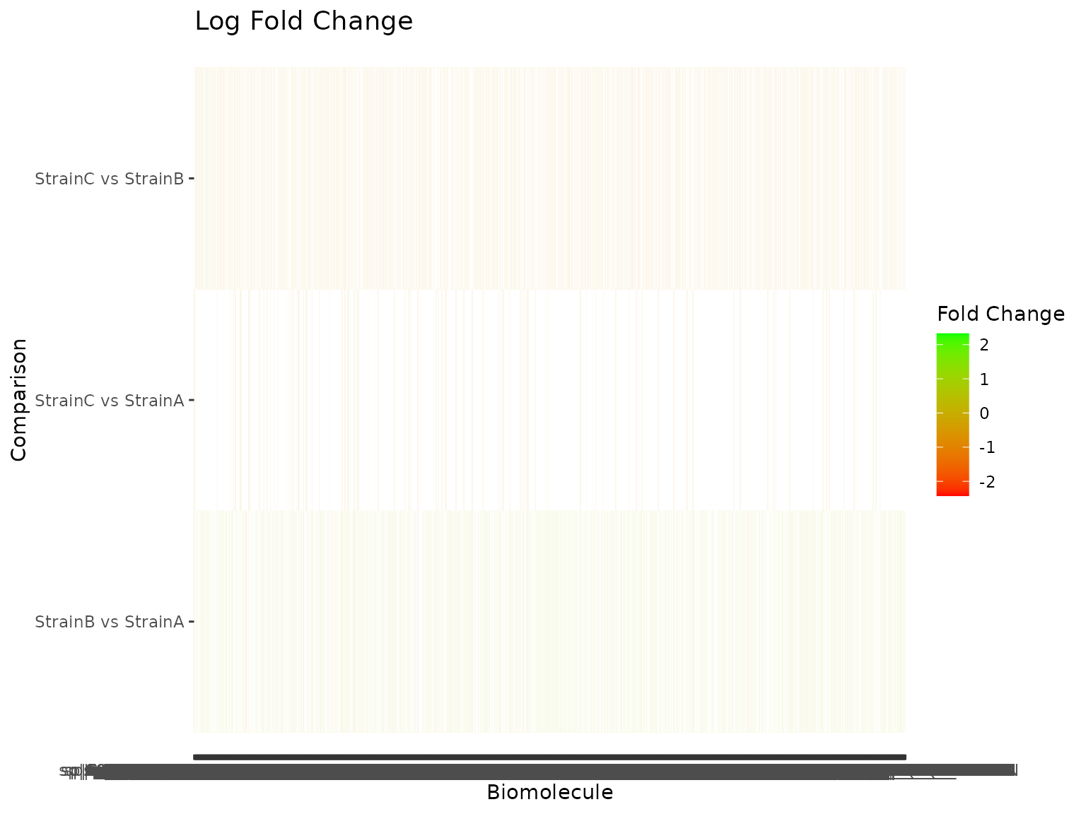
See ?imd_anova for more details and options.