RNAseq Data Processing
Kelly Stratton, Rachel Richardson, Lisa Bramer
2025-10-22
Source:vignettes/RNAseq_Processing_Workflow.Rmd
RNAseq_Processing_Workflow.RmdOverview
RNAseq data in pmartR follows a different workflow
compared to the other data types, with different filtering, plotting,
and statistical options. This vignette walks through the RNAseq workflow
using example data from the pmartRdata package, including
the use of all three statistical analysis options, DEseq2 (Love, Anders, and Huber 2014), edgeR (Robinson, McCarthy, and Smyth 2010), or
limmaVOOM (Law et al. 2014).
Data Set-up
Data upload, create object
For these data, the column named “Transcript” denotes the transcript identifier in e_data.
head(edata)## Transcript StrainC_2_A StrainC_2_B StrainC_2_C StrainC_2_D StrainC_2_E
## 1 ENSG00000223972 0 0 0 0 0
## 2 ENSG00000227232 109 65 77 76 100
## 3 ENSG00000278267 14 12 6 1 11
## 4 ENSG00000243485 0 0 0 0 0
## 7 ENSG00000240361 0 0 0 0 0
## 9 ENSG00000238009 0 0 0 1 0
## StrainA_2_A StrainA_2_B StrainA_2_C StrainA_2_D StrainA_2_E StrainC_3_A
## 1 0 0 0 0 0 0
## 2 83 83 61 58 61 80
## 3 11 14 10 13 6 9
## 4 0 0 0 1 1 2
## 7 0 0 0 0 0 0
## 9 2 0 0 3 3 0
## StrainC_3_B StrainC_3_C StrainC_3_D StrainC_3_E StrainA_3_A StrainA_3_B
## 1 0 0 0 0 0 0
## 2 101 76 68 86 76 57
## 3 8 8 12 1 2 3
## 4 0 1 0 0 1 0
## 7 0 0 0 0 0 0
## 9 0 4 0 0 1 0
## StrainA_3_C StrainA_3_D StrainA_3_E StrainC_1_A StrainC_1_B StrainC_1_C
## 1 1 0 0 2 0 0
## 2 56 32 72 98 132 102
## 3 10 1 15 11 12 9
## 4 0 0 1 1 0 0
## 7 0 0 0 0 0 0
## 9 0 1 2 2 0 1
## StrainC_1_D StrainC_1_E StrainA_1_A StrainA_1_B StrainA_1_C StrainA_1_D
## 1 0 0 0 0 0 0
## 2 51 60 81 52 48 48
## 3 2 8 15 6 5 3
## 4 0 1 0 2 1 1
## 7 0 0 0 0 0 0
## 9 3 11 0 0 0 0
## StrainA_1_E StrainB_3_A StrainB_3_B StrainB_3_C StrainB_3_D StrainB_3_E
## 1 0 0 0 0 0 2
## 2 64 52 48 64 51 87
## 3 1 6 3 2 2 7
## 4 0 0 0 0 2 0
## 7 0 0 0 0 0 0
## 9 0 1 3 3 6 4
## StrainB_2_A StrainB_2_B StrainB_2_C StrainB_2_D StrainB_2_E StrainB_1_A
## 1 0 0 0 0 0 0
## 2 72 97 83 119 84 53
## 3 3 5 10 5 15 1
## 4 0 0 0 0 1 0
## 7 0 0 0 0 0 1
## 9 1 1 2 2 1 1
## StrainB_1_B StrainB_1_C StrainB_1_D StrainB_1_E
## 1 1 0 0 0
## 2 91 76 84 78
## 3 4 5 3 6
## 4 0 0 0 0
## 7 0 0 0 0
## 9 0 0 2 0The f_data data frame contains the sample identifier, “SampleName”, mapping to the column names in e_data other than “Transcript”. The column for “Virus” takes on 1 of 3 values, and will be used as our main effect, since comparisons of interest in this experiment are between virus strains. Finally, f_data contains information about the Donor and Replicate, which describe the provenance of the samples and biological replicate information.
head(fdata)## SampleName Virus Replicate Donor
## 34 StrainC_2_A StrainC A 2
## 40 StrainC_2_B StrainC B 2
## 46 StrainC_2_C StrainC C 2
## 52 StrainC_2_D StrainC D 2
## 58 StrainC_2_E StrainC E 2
## 64 StrainA_2_A StrainA A 2The e_meta data frame contains just 2 columns, “Transcript” and “Gene”. The “Transcript” column contains the same transcripts found in e_data, and “Gene” provides the mapping of the transcripts to the gene level.
head(emeta)## Transcript Gene
## 1 ENSG00000223972 DDX11L1
## 2 ENSG00000227232 WASH7P
## 3 ENSG00000278267 MIR6859-1
## 4 ENSG00000243485 MIR1302-2HG
## 5 ENSG00000237613 FAM138A
## 6 ENSG00000268020 OR4G4PSince these are RNAseq data, we will create a seqData
object in pmartR. Note that unlike the other data types
supported in pmartR, seqData objects are not log2
transformed.
myseq <- as.seqData(
  e_data = rnaseq_edata,
  e_meta = rnaseq_emeta,
  f_data = rnaseq_fdata,
  edata_cname = "Transcript",
  fdata_cname = "SampleName",
  emeta_cname = "Transcript"
)
## Warning in pre_flight(e_data = e_data, f_data = f_data, e_meta = e_meta, :
## Extra RNA transcripts were found in e_meta that were not in e_data. These have
## been removed from e_meta.We can use the summary function to get basic summary
information for our isbaricseqData object.
summary(myseq)##
## Class seqData
## Unique SampleNames (f_data) 45
## Unique Transcripts (e_data) 49568
## Unique Transcripts (e_meta) 49568
## Observed Zero-Counts 872181
## Proportion Zeros 0.391Using the plot function on our seqData object provides
box plots of log counts per million (lcpm) for each sample.
plot(myseq, transformation = "lcpm")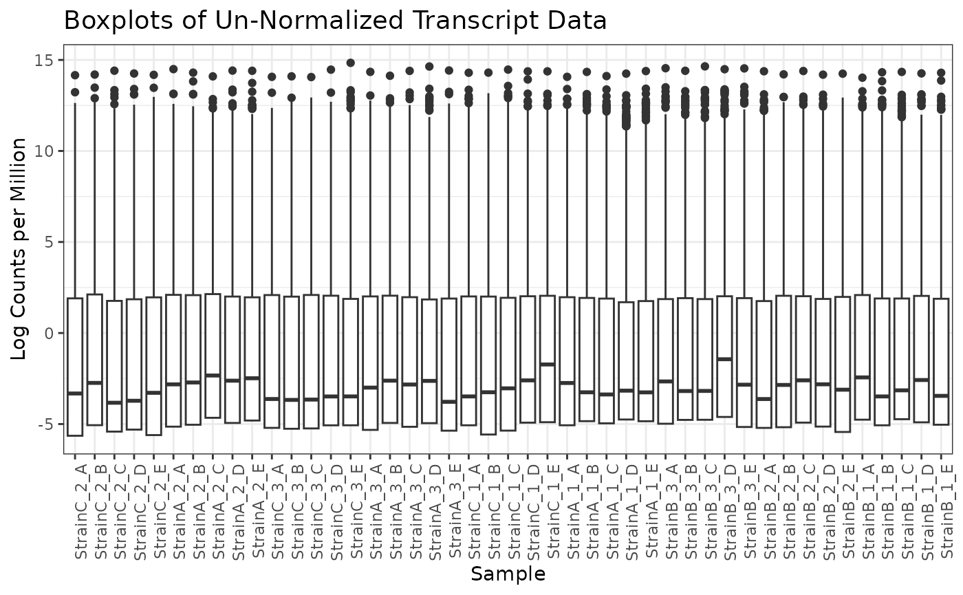
Workflow
Main Effects
We are preparing this data for statistical analysis where we will
compare the samples belonging to one group to the samples belonging to
another, and so we must specify the group membership of the samples. We
do this using the group_designation() function, which
modifies our seqData object and returns an updated version of it. Up to
two main effects and up to two covariates may be specified (VERIFY THIS
IS TRUE), with one main effect being required at minimum. For these
example data, we specify the main effect to be “Virus” so that we can
make comparisons between the different strains. Certain functions we
will use below require that groups have been designated via the
group_designation() function, and doing so makes the
results of plot and summary more
meaningful.
myseq <- group_designation(omicsData = myseq, main_effects = "Virus")
summary(myseq)
##
## Class seqData
## Unique SampleNames (f_data) 45
## Unique Transcripts (e_data) 49568
## Unique Transcripts (e_meta) 49568
## Observed Zero-Counts 872181
## Proportion Zeros 0.391
## Samples per group: StrainC 15
## Samples per group: StrainA 15
## Samples per group: StrainB 15
plot(myseq, order_by = "Virus", color_by = "Virus", transformation = "lcpm")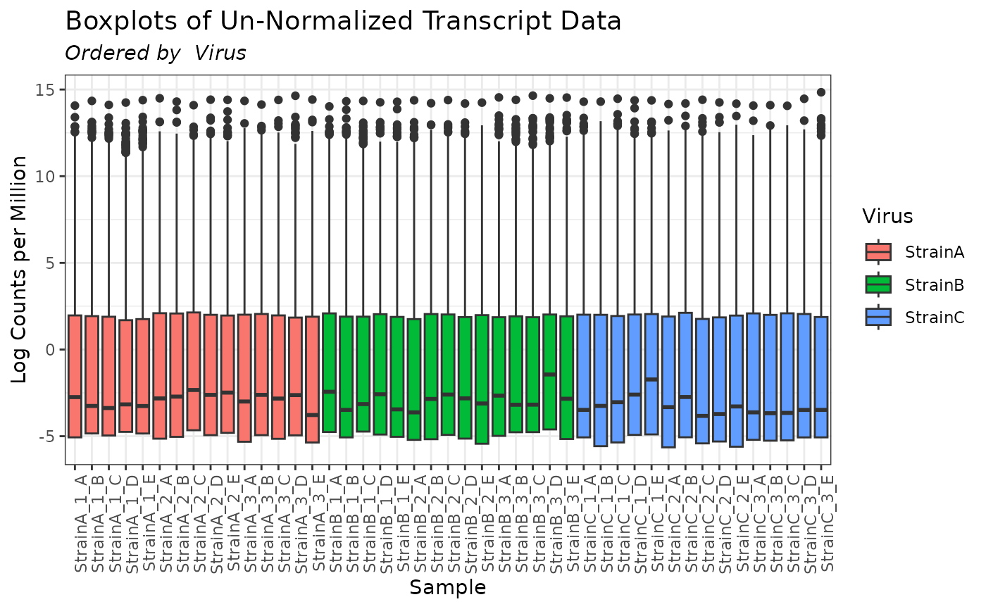
The group_designation() function creates an attribute of
the dataset as follows:
attributes(myseq)$group_DF## SampleName Group
## 1 StrainC_2_A StrainC
## 2 StrainC_2_B StrainC
## 3 StrainC_2_C StrainC
## 4 StrainC_2_D StrainC
## 5 StrainC_2_E StrainC
## 6 StrainA_2_A StrainA
## 7 StrainA_2_B StrainA
## 8 StrainA_2_C StrainA
## 9 StrainA_2_D StrainA
## 10 StrainA_2_E StrainA
## 11 StrainC_3_A StrainC
## 12 StrainC_3_B StrainC
## 13 StrainC_3_C StrainC
## 14 StrainC_3_D StrainC
## 15 StrainC_3_E StrainC
## 16 StrainA_3_A StrainA
## 17 StrainA_3_B StrainA
## 18 StrainA_3_C StrainA
## 19 StrainA_3_D StrainA
## 20 StrainA_3_E StrainA
## 21 StrainC_1_A StrainC
## 22 StrainC_1_B StrainC
## 23 StrainC_1_C StrainC
## 24 StrainC_1_D StrainC
## 25 StrainC_1_E StrainC
## 26 StrainA_1_A StrainA
## 27 StrainA_1_B StrainA
## 28 StrainA_1_C StrainA
## 29 StrainA_1_D StrainA
## 30 StrainA_1_E StrainA
## 31 StrainB_3_A StrainB
## 32 StrainB_3_B StrainB
## 33 StrainB_3_C StrainB
## 34 StrainB_3_D StrainB
## 35 StrainB_3_E StrainB
## 36 StrainB_2_A StrainB
## 37 StrainB_2_B StrainB
## 38 StrainB_2_C StrainB
## 39 StrainB_2_D StrainB
## 40 StrainB_2_E StrainB
## 41 StrainB_1_A StrainB
## 42 StrainB_1_B StrainB
## 43 StrainB_1_C StrainB
## 44 StrainB_1_D StrainB
## 45 StrainB_1_E StrainBFilter Biomolecules
Transcripts can be removed from seqData objects using
the molecule filter or the custom filter, if desired. See the “Filter
Functionality” vignette for more information.
Total Count Filter
The total count filter is specifically applicable to
seqData objects, and is implemented in pmartR
based on recommendations in edgeR processing (Robinson, McCarthy, and Smyth 2010), where the
low-observed biomolecules are removed. Here we use the default
recommendation in edgeR and require at least 15 total counts observed
across samples. We plot the filter first without a
min_count threshold, and then with our threshold of 15, so
we can see how the application of the filter changes the observation
density.
mytotcountfilt <- total_count_filter(omicsData = myseq)
summary(mytotcountfilt, min_count = 15)
##
## Summary of Total Count Filter
## ----------------------
## Counts:
##
## Min. 1st Qu. Median Mean 3rd Qu. Max.
## 1 14 79 15477 3194 15803184
##
## Number Filtered Biomolecules: 12765
plot(mytotcountfilt)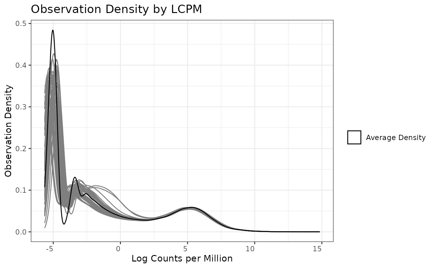
plot(mytotcountfilt, min_count = 15)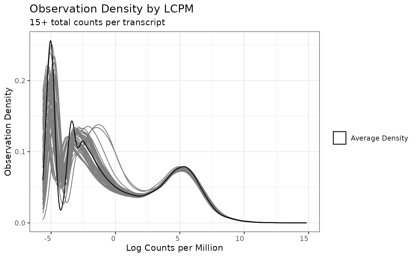
Once we are satified with the filter results, we apply the filter to
the seqData object.
myseq <- applyFilt(filter_object = mytotcountfilt, omicsData = myseq, min_count = 15)Filter Samples
RNA Filter: Total Library Size Filter
The RNA filter removes samples based on either:
library size (number of reads)
number/proportion of unique non-zero biomolecules per sample
This filter is particularly useful for identifying any samples that contain lower than expected numbers of reads.
First we utilize this filter to identify any samples with fewer than one million reads, of which there are none.
# create RNA filter object
myrnafilt <- RNA_filter(omicsData = myseq)

# filter by library size
plot(myrnafilt, plot_type = "library")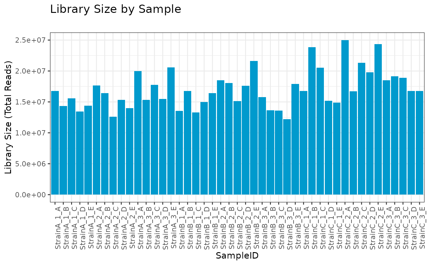
plot(myrnafilt, plot_type = "library", size_library = 1000000)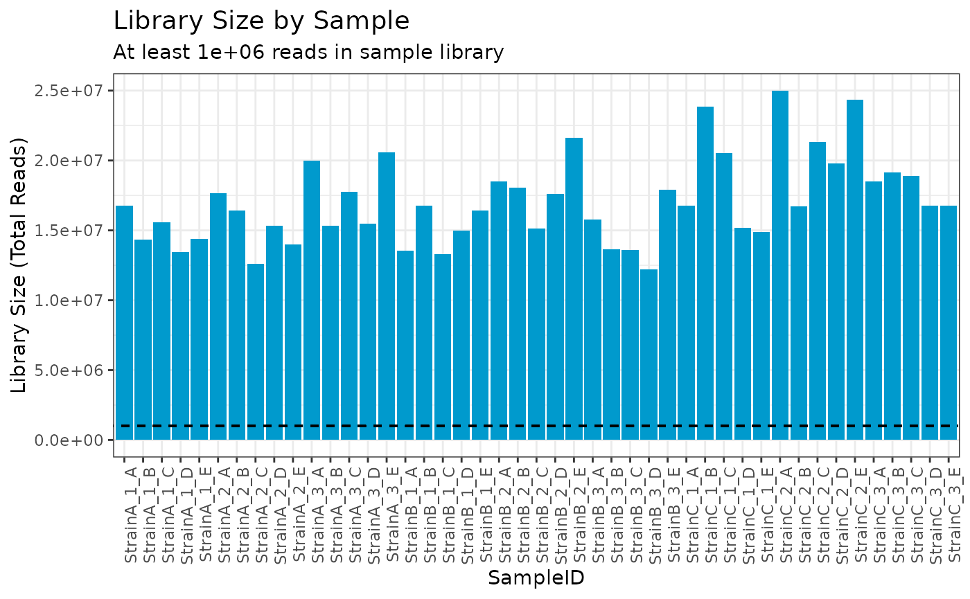
Next, we utilize the filter to identify any samples with fewer than 5,000 non-zero counts, of which there are none.
# filter based on number or proportion of non-zero counts
plot(myrnafilt, plot_type = "biomolecule", min_nonzero = 5000)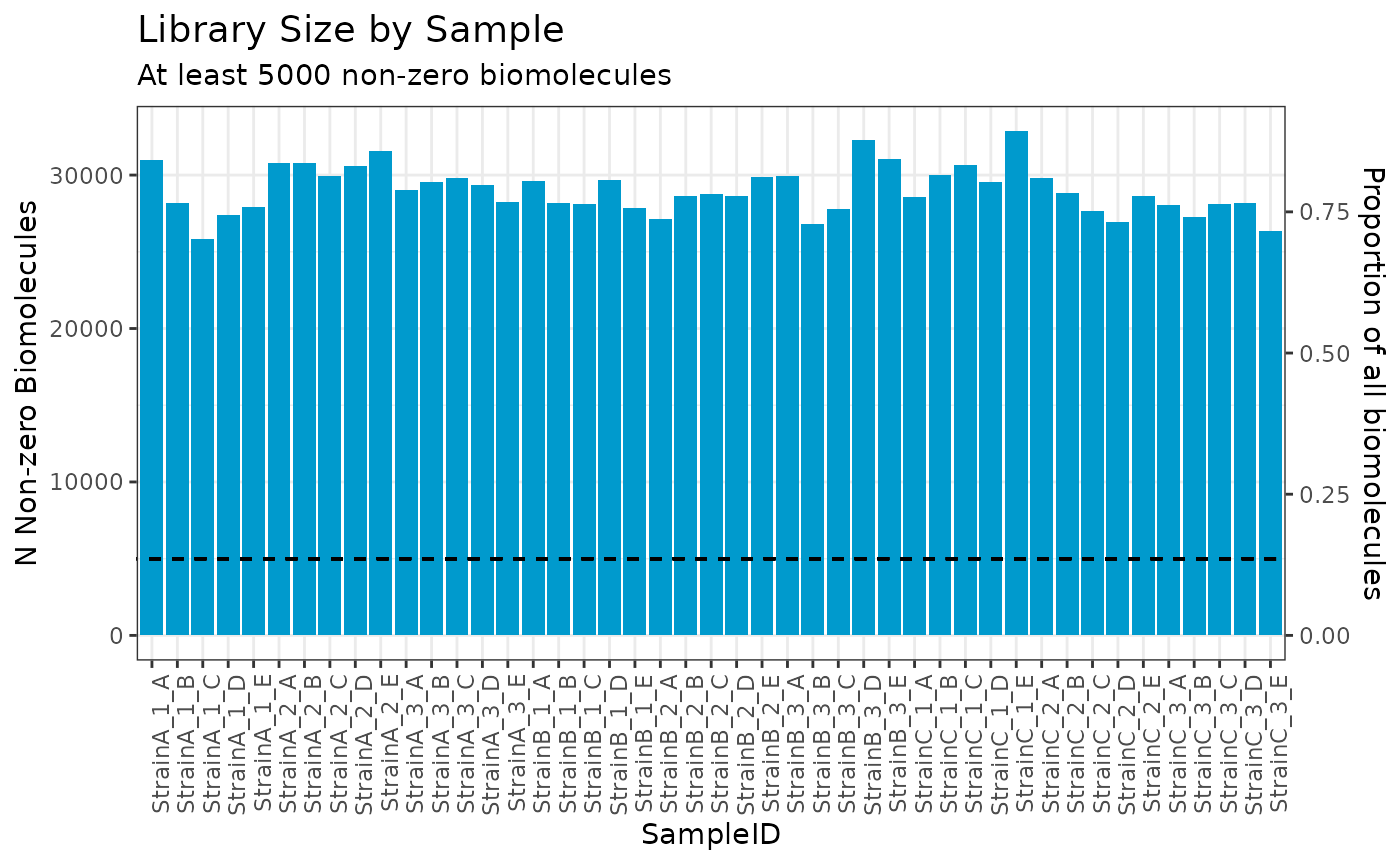
Summarize Data
After filtering out any transcripts and/or samples above, we may wish to do some exploratory data analysis.
Correlation Heatmap
A Spearman correlation heatmap shows a couple of samples with lower correlation than the rest, but neither of these are
Strain B 3 D
Strain C 1 E
mycor <- cor_result(omicsData = myseq)
plot(mycor, interactive = TRUE)
Principal Components Analysis
A principal components analysis (GLM-PCA) plot of our data shows clustering of strains A and C with one another, separated from strain B. The two samples that are separated on PC1 one from the rest are the same two samples that stood out in the correlation heatmap. Note: Randomness is present in GLM-PCA computations, set.seed() can be used to ensure consistent results.
set.seed(2025)
mypca <- dim_reduction(omicsData = myseq, k = 2)
plot(mypca, interactive = TRUE)
mypca_df <- data.frame(check.names = FALSE, SampleID = mypca$SampleID, PC1 = mypca$PC1, PC2 = mypca$PC2)Normalization & Statistical Comparisons
For RNAseq data there are three methods available via
pmartR for making statistical comparisons:
edgeR (Robinson, McCarthy, and Smyth 2010)
DESeq2 (Love, Anders, and Huber 2014)
limma-voom (Law et al. 2014)
Here we utilize all three for demonstration purposes, but in practice
a single method should be utilized, the selection of which can be guided
by visual inspection of dispersion plots for each method via
dispersion_est. After using the diffexp_seq
function to perform statistical comparisons with the selected method,
plot and summary methods are available to help
display the results, and the data frame returned by the
diffexp_seq function can be saved as an Excel file or
another useful format if helpful.
edgeR Method
We examine the dispersion plot for use of the edgeR method.
dispersion_est(omicsData = myseq, method = "edgeR")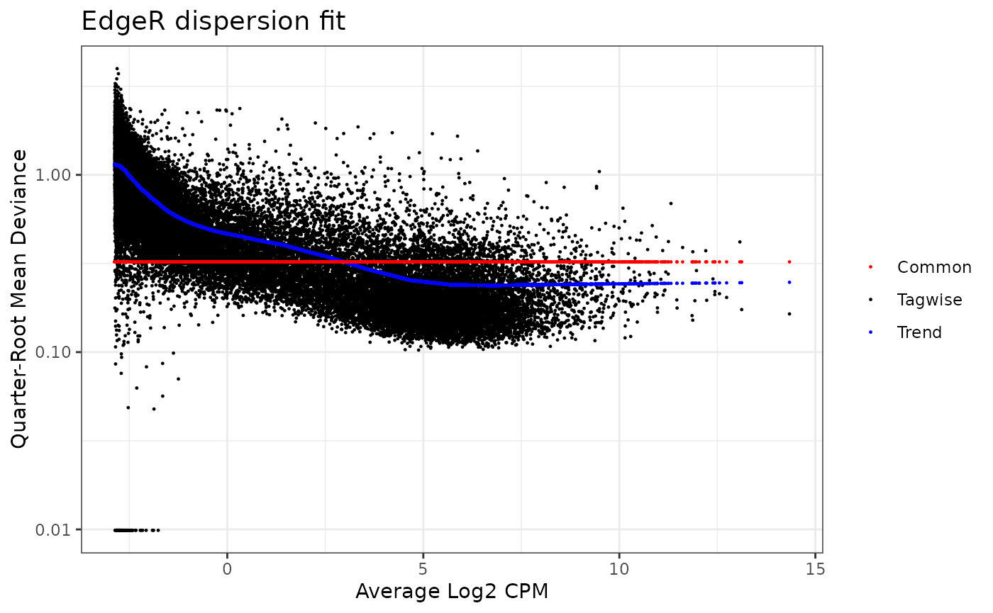
If we are satisfied with using this method for our statistical comparisons between virus strains, we can do so as follows.
stats_edger <- diffexp_seq(omicsData = myseq, method = "edgeR")## Joining with `by = join_by(Transcript, NonZero_Count_StrainC)`
## Joining with `by = join_by(Transcript, NonZero_Count_StrainA,
## NonZero_Count_StrainB)`Various plot types are available to display the results of the statistical comparisons.
plot(stats_edger, plot_type = "volcano")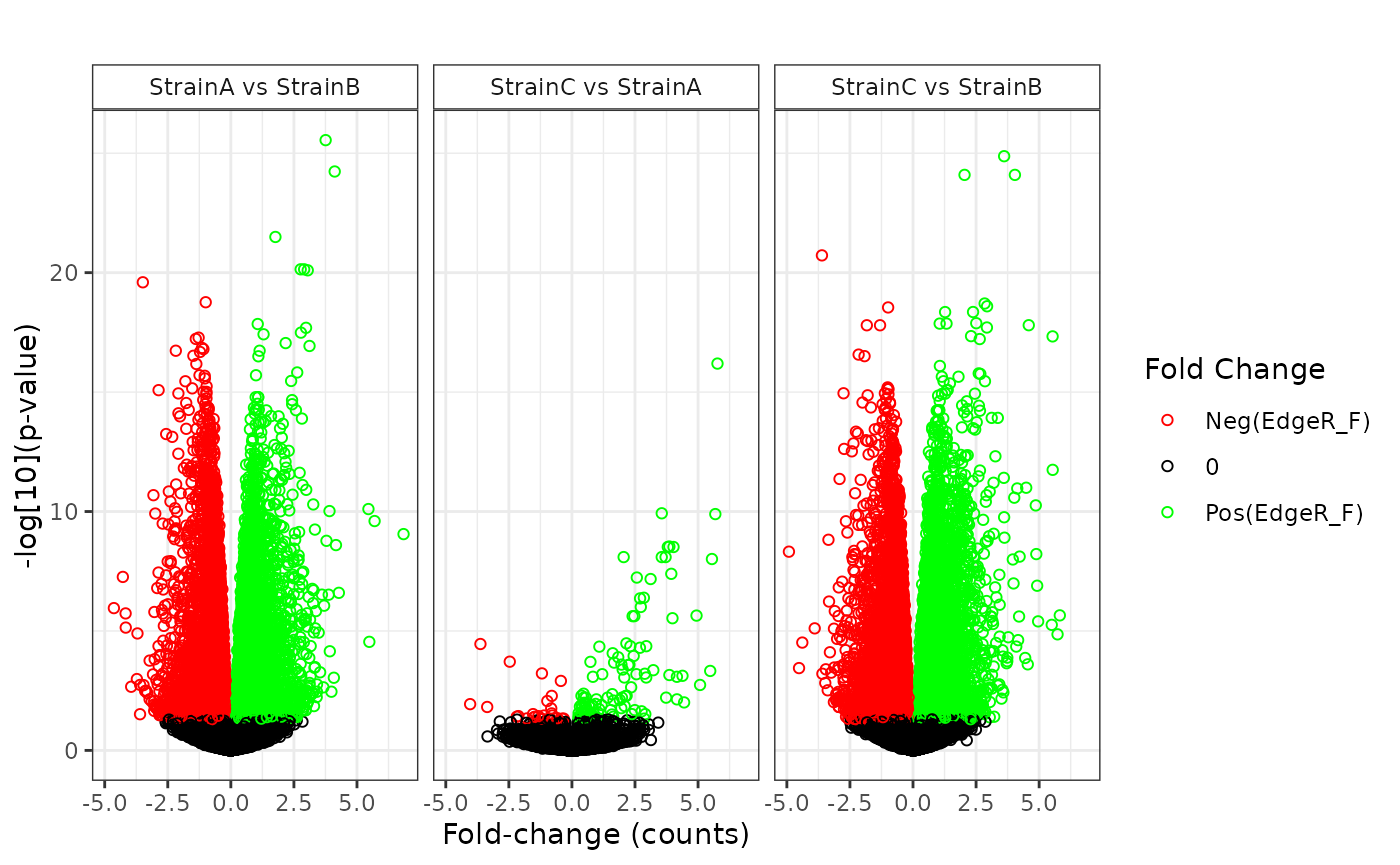
plot(stats_edger, plot_type = "bar")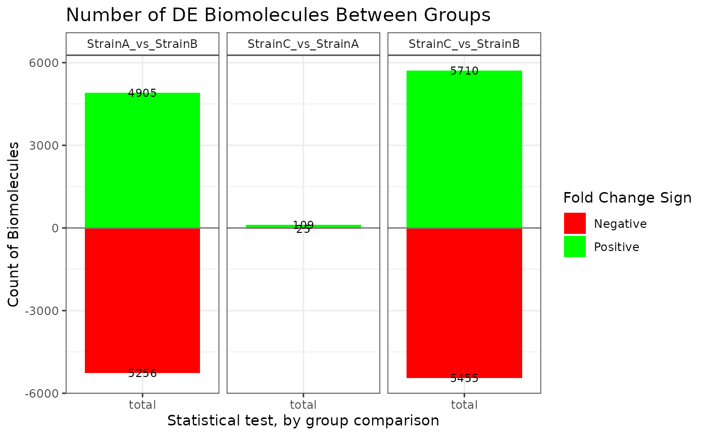
plot(stats_edger, plot_type = "ma")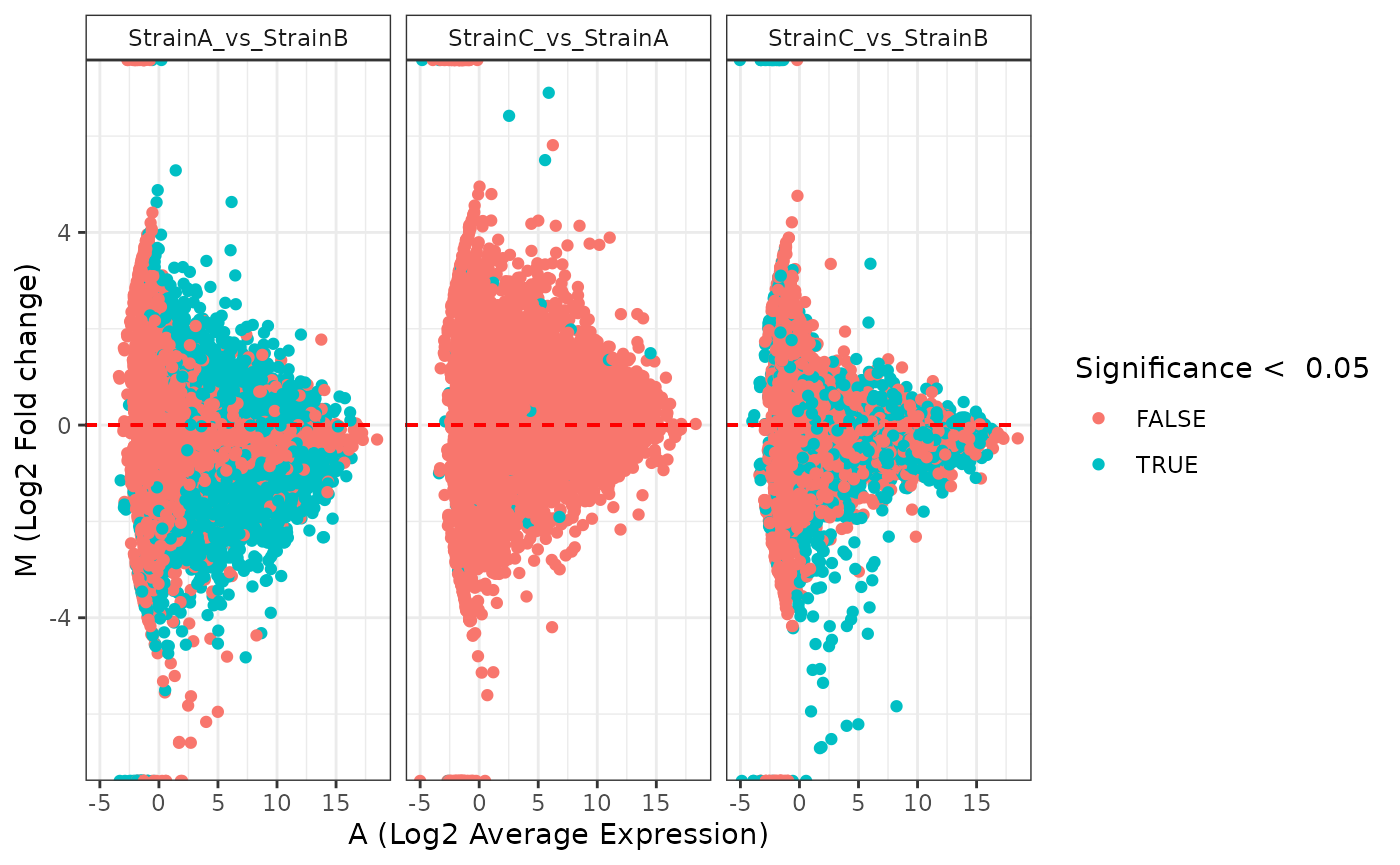
DESeq2 Method
We examine the dispersion plot for use of the DESeq2 method.
dispersion_est(omicsData = myseq, method = "DESeq2")## gene-wise dispersion estimates## mean-dispersion relationship## final dispersion estimates## Warning in as.data.frame.DataFrame(check.names = FALSE, S4Vectors::mcols(dds)):
## arguments in '...' ignored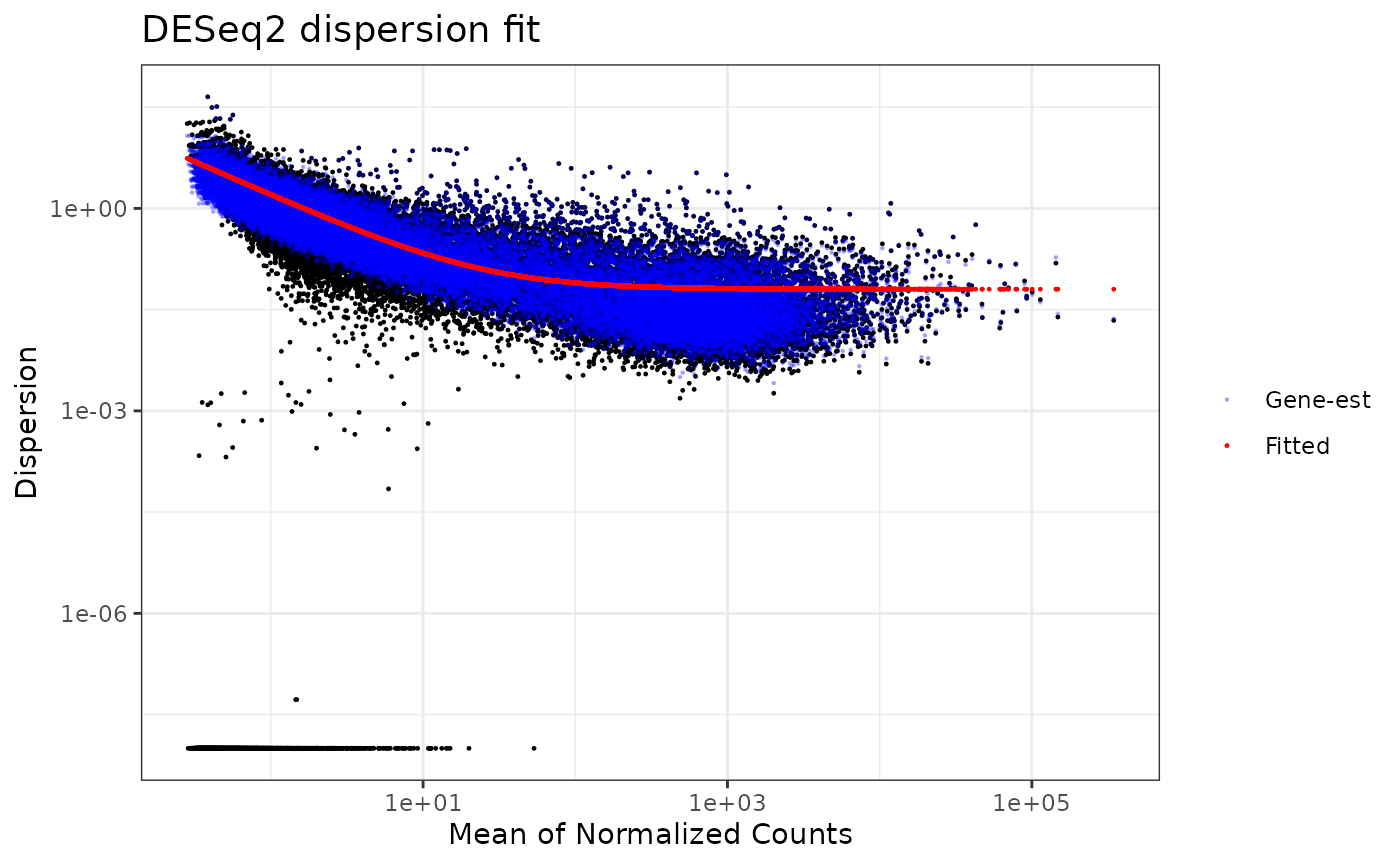
If we are satisfied with using this method for our statistical comparisons between virus strains, we can do so as follows.
stats_deseq <- diffexp_seq(omicsData = myseq, method = "DESeq2")## Joining with `by = join_by(Transcript, NonZero_Count_StrainC)`
## Joining with `by = join_by(Transcript, NonZero_Count_StrainA,
## NonZero_Count_StrainB)`Various plot types are available to display the results of the statistical comparisons.
plot(stats_deseq, plot_type = "volcano")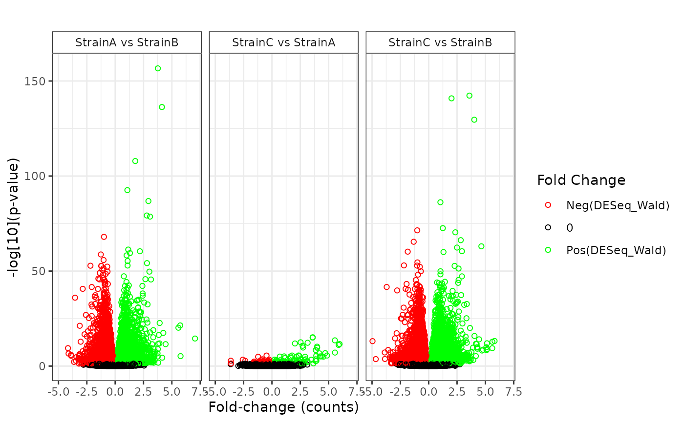
plot(stats_deseq, plot_type = "bar")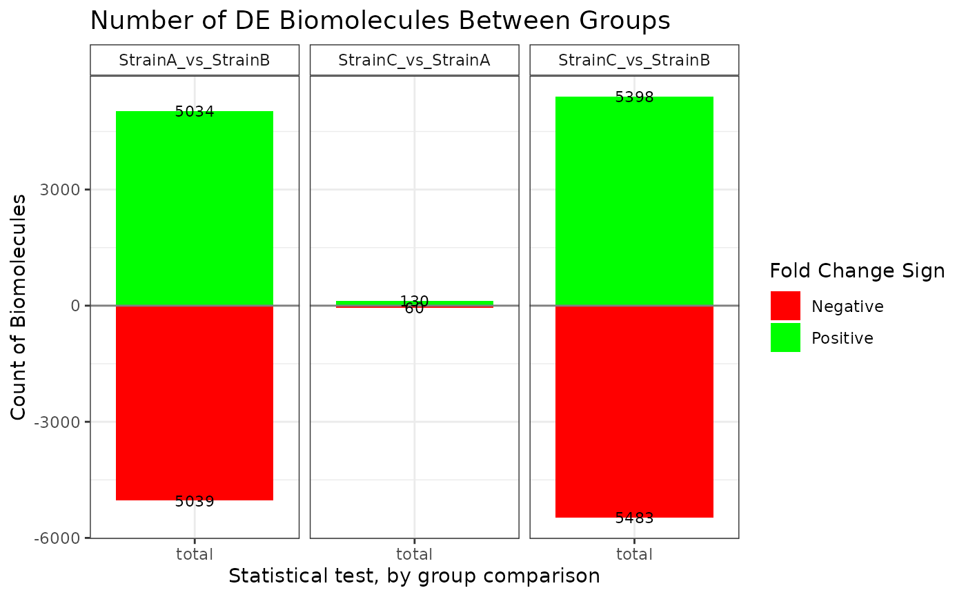
plot(stats_deseq, plot_type = "ma")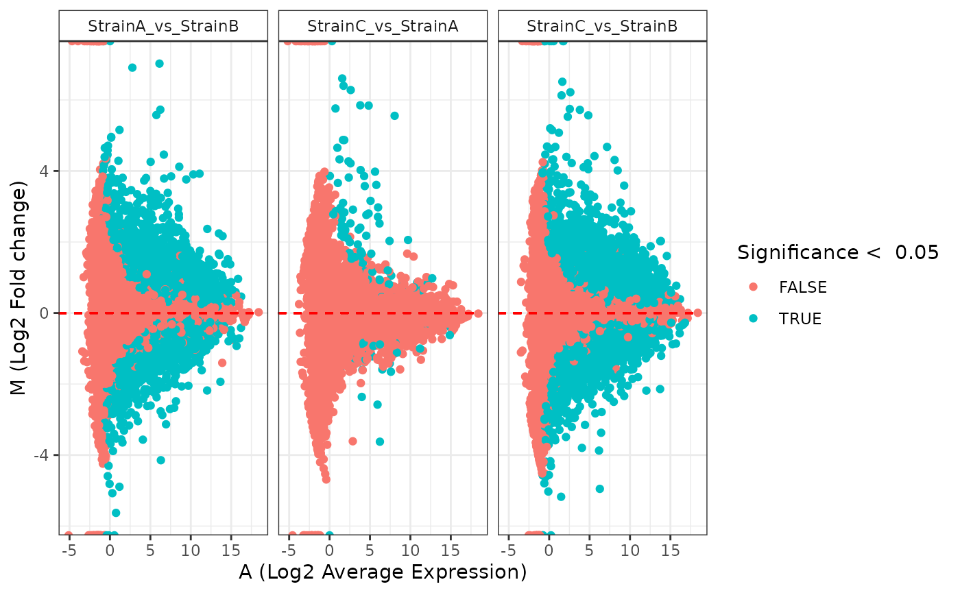
limma-voom Method
We examine the dispersion plot for use of the voom method.
dispersion_est(omicsData = myseq, method = "voom")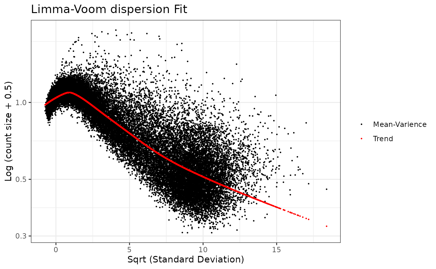
If we are satisfied with using this method for our statistical comparisons between virus strains, we can do so as follows.
stats_voom <- diffexp_seq(omicsData = myseq, method = "voom")## Joining with `by = join_by(Transcript, NonZero_Count_StrainC)`
## Joining with `by = join_by(Transcript, NonZero_Count_StrainA,
## NonZero_Count_StrainB)`Various plot types are available to display the results of the statistical comparisons.
plot(stats_voom, plot_type = "volcano")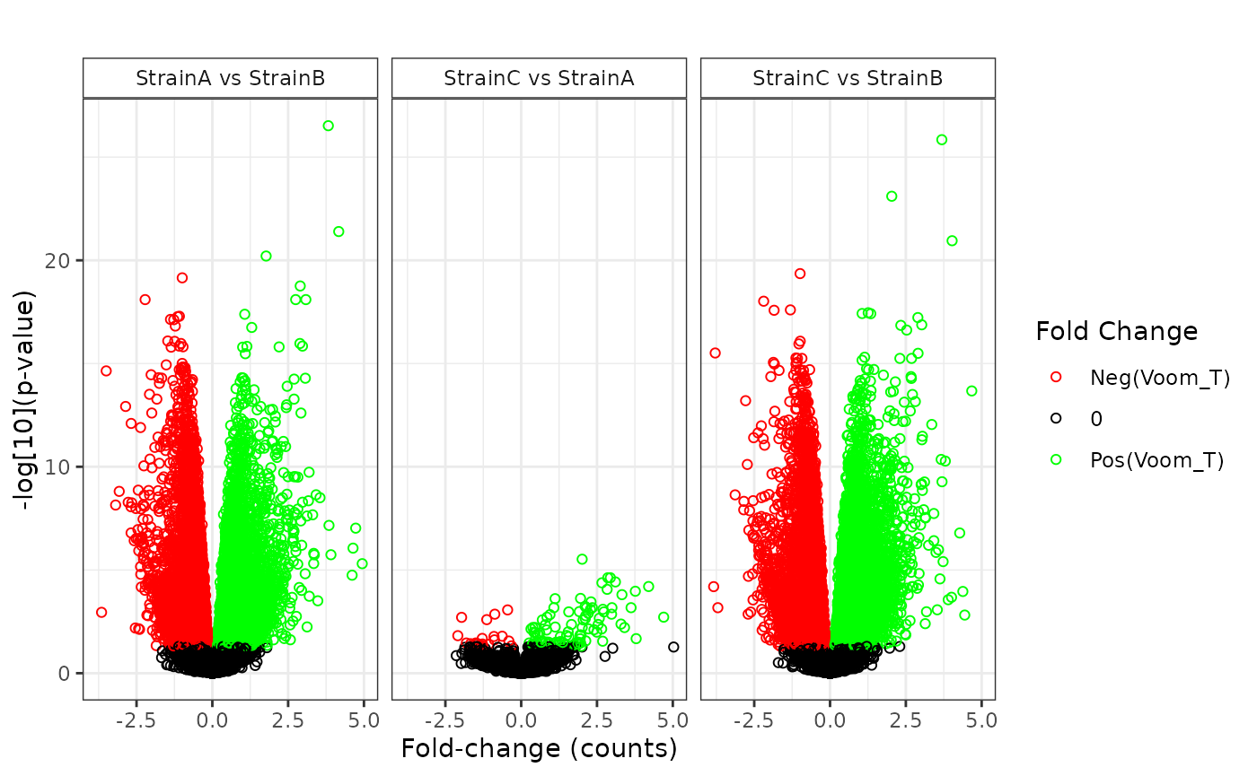
plot(stats_voom, plot_type = "bar")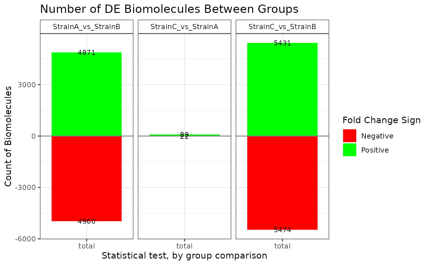
plot(stats_voom, plot_type = "ma")