Statistical Analysis with the `pmartR` Package

library(pmartR)
library(pmartRdata)

pep_object <- edata_transform(
  omicsData = pmartRdata::pep_object,
  data_scale = "log2"
)

Introduction

This vignette describes the statistical analysis capabilities for omicsData objects other than seqData. For details about the statistical methods for seqData objects, see ?diffexp_seq.

The pmartR package includes functions to assess qualitative and quantitative differences in abundance data using the IMD-ANOVA method described in Webb-Robertson et al. (2010). Our IMD-ANOVA functionality can handle omics datasets with various experimental designs, including up to two grouping factors with or without additional covariate information. The data can be paired or not.

The functionality of the pmartR package will be illustrated with peptide data available from the pmartRdata package called pep_object. In a nutshell, the pep_object object is a list of length three of the class pepData. The e_data element contains all of the peptide abundance data, the f_data object contains sample information, and the e_meta object contains meta information related to the peptides in the dataset. See ?pmartRdata for more on this data set.

IMD-ANOVA Test for Differential Abundance

The imd_anova() function is used to implement the IMD test, ANOVA test, or combined IMD-ANOVA test. Using the combined test simply means that both ANOVA and IMD are used, and results reported for both tests.

Below, descriptions of ANOVA and IMD are provided, followed by a description of the output from the imd_anova() function.

Analysis of Variance

Quantitative tests for differential abundance of pan-omic data are accomplished using the function test_method = "anova" or test_method = "combined" arguments, which implement an analysis of variance (ANOVA) for each biomolecule. Rcpp and parallel processing are used to speed up computation (Eddelbuettel (2013)). Different ANOVA implementations are applied depending on the complexity of the supplied data. For example, if only two groups are supplied then ANOVA reduces to a two sample $t$ -test that assumes equal variance for the two groups. Alternatively, if two groups are present and a covariate correction is required, then a two-factor ANCOVA is used to detect differences between all combinations of groups or between main effects as appropriate controlling for covariates. Details on generalizations to these two approaches are given in the next two subsections.

One Group

If there is only one grouping factor and that factor has more than two levels, then a one-way ANOVA tests for quantitative differences between the groups. Let $y_{ik}$ represent the biomolecule abundance for observation $k=1,\dots,n_i$ in group $i=1,\dots,m$ on the log base 2 scale then we assume $\begin{equation} y_{ik}=\mu_i+\epsilon_{ik} \label{eq:one_group} \end{equation}$ where $\mu_i$ represents the mean abundance of group $i$ (on the log-scale) and $\epsilon_{ik}$ are the error terms that are assumed to be independent and identically distributed (iid) according to the normal distribution with mean $0$ and variance $\sigma^2$ . Group comparisons are performed according to 3.1 General linear models in (Bretz, Hothorn, and Westfall (2016)). Under the hood, a linear model of the form $\mathbf{y} = \mathbf{X}\mathbf{\beta} + \epsilon$ is fit, and the design matrix is used to form the appropriate contrast matrix for comparing means. This framework extends to the two factor case as well.

The code below will group the peptide data by Phenotype, which is a categorical variable with three levels: “Phenotype1”, “Phenotype2”, and “Phenotype3”. Then the anova_test function fits the model described above and tests for differential abundance between each pair of phenotypes for every peptide.

pep_object <- group_designation(
  omicsData = pep_object,
  main_effects = c("Phenotype")
)
myfilt <- imdanova_filter(omicsData = pep_object)
pep_object <- applyFilt(
  filter_object = myfilt,
  omicsData = pep_object,
  min_nonmiss_anova = 2,
  min_nonmiss_gtest = 3
)
all_pairwise_results <- imd_anova(
  omicsData = pep_object,
  test_method = "anova"
)

The function imd_anova function returns a data frame containing:

The number of observed values in each group in the columns called Count_i where i is replaced by the group name supplied as an attribute of the omicsData argument,
The least squares means for each group in the columns called Mean_i where i is replaced by the group name supplied as an attribute of the omicsData argument,
The $p$ -values for each comparison in the columns called P_value_A_ (“A” for ANOVA)
The (log2) fold change for each comparison,
An indicator for significance for each comparison in the columns called Flag_A_ (“A” for ANOVA) that is a $\pm1$ or 0 depending on whether that fold change was or was not statistically significant from zero, respectively, according to the $p$ -values and the specified $p$ -value threshold set by the pval_thresh argument to imd_anova. A value of $-1$ implies the “control” or “reference” group is significantly under expressed compared to the test group, and the converse is true for $+1$ .

The $p$ -values associated with each group comparison can be adjusted for multiple comparisons using the pval_adjust_a_multcomp argument to imd_anova. A detailed look at the available $p$ -value adjustment methods and when they should be applied are discussed later in this vignette, but the use of the Tukey multiple comparison method is illustrated in the following.

all_pairwise_results_adjusted <- imd_anova(
  omicsData = pep_object,
  test_method = "anova",
  pval_adjust_a_multcomp = "Tukey"
)

By default, all pairwise comparisons are made. Custom comparisons can by defined by passing a data.frame to the comparisons argument with column names “Test” and “Control”. Now, group “Phenotype1” is treated as the control group and the remaining groups are compared to it.

one_vs_all <- data.frame(
  Control = rep("Phenotype1", 2),
  Test = c("Phenotype2", "Phenotype3")
)
one_vs_all_results <- imd_anova(
  omicsData = pep_object,
  test_method = "anova",
  comparisons = one_vs_all
)

If the grouping variable has only two levels, $m=2$ , then a Welch’s $t$ -test is performed instead of an ANOVA. That is, the model defined in equation () is still fit, but the two groups of the grouping factor are allowed to have different variances. In particular, the error terms $\epsilon_{ik}$ are assumed to be independently distributed according to the normal distribution with mean $0$ and variance $\sigma^2_i$ . To determine if the biomolecules are differentially expressed, $p$ -values are derived from a $t$ -distribution with degrees of freedom approximated by the Satterthwaite equation. The value for Variance, which is not a pooled variance estimate, scaled by the Satterthwaite approximate degrees of freedom. To illustrate this the data are grouped by “SecondPhenotype”, which has two values, then fit with ANOVA.

pep_object <- group_designation(
  omicsData = pep_object,
  main_effects = c("SecondPhenotype")
)
all_pairwise_results <- imd_anova(
  omicsData = pep_object,
  test_method = "anova"
)

When this model is fit, it is imperative the researcher check the assumptions of the model. In particular for the $m>2$ case, the residuals $\hat \epsilon_{ik}=y_{ik}-\hat \mu_i$ are assumed to be independent, normally distributed and have a common variance across groups. The appropriateness of this assumption can be assessed using quantile-quantile plots and comparisons of each group’s variance.

Two Groups

Next we consider the case where there are two grouping factors again in the context of biomolecule abundance. Let $y_{ijk}$ represent the biomolecule abundance for observation $k=1,\dots,n_{ij}$ in group $i=1,\dots,m$ and group $j=1,\dots,p$ on the log base 2 scale then we assume $\begin{equation} y_{ijk}=\mu_i+\alpha_j+\gamma_{ij}+\epsilon_{ijk} \label{eq:full_model} \end{equation}$ where $\mu_i+\alpha_j+\gamma_{ij}$ represents the mean abundance for an observation in $i$ th first group and $j$ th second group which have marginal means $\mu_i$ and $\alpha_j$ , respectively. Finally, $\gamma_{ij}$ is the interaction effect of group $ij$ , and $\epsilon_{ijk}$ are the error terms that are assumed to be iid according to the normal distribution with mean $0$ and variance $\sigma^2$ .

For each biomolecule, the test_method = "anova" argument automatically tests if the $\gamma_{ij}$ effect is statistically significant from zero using a full and reduced model $F$ -test. That is, in addition to the model above, the reduced model $\begin{equation} y_{ijk}=\mu_i+\alpha_j+\epsilon_{ijk} \label{eq:red_model} \end{equation}$ is also fit and the test statistic $F^*=\frac{MSE_F}{(SSE_R-SSE_F)/(df_R-df_F)}$ is computed where $MSE_\cdot$ and $df_\cdot$ are the mean square error and degrees of freedom for the full (F; ) or reduced (R; ) model, respectively. A $p$ -value is computed based on $F^*$ as $p=P(F^*>F_{a,b})$ where $F_{a,b}$ is compared to an $F$ distribution with degrees of freedom $a=df_F$ and $b=df_R-df_F$ . If $p<0.05$ then there is significant evidence to reject the null hypothesis that the reduced model is adequate and the full model is used to test for group differences. Conversely, if $p\geq 0.05$ then there is not enough evidence to reject the null hypothesis and the reduced model is used. Group comparisons are computed in the same manner as the one-factor case, following 3.1 General linear models in (Bretz, Hothorn, and Westfall (2016)).

Regardless of whether the full or reduced model is used, both assume that the residuals are independent and normally distributed with a common variance for all groups. These assumptions must be checked before the results of the model are used to assess differential abundance.

Covariate Adjustment

If, in addition to a single grouping factor, there are covariates to account for when testing for differential abundance then a linear model of the form $\begin{equation} \mathbf{y}=\mathbf{X} \beta_1+\mathbf{V} \beta_2 + \epsilon \label{eq:covar_adj} \end{equation}$ is fit to the transformed abundance data $\mathbf{y}$ where $\mathbf{X}$ is the dummy-encoded design matrix for the main effects, $\mathbf{V}$ is the design matrix for any covariates, $\beta_1$ and $\beta_2$ are the parameters to be estimated for the main effects and covariates, and $\epsilon$ is the error term. Note that $\mathbf{X}$ allows for the one factor model, as well as the full and reduced forms of the two factor model. We estimate the least squares means using the estimated coefficients $\beta_1$ and $\beta_2$ . Specifically, when computing the the least squares mean for a particular combination of main effect levels, we consider the predicted value of the fitted model at the main effect levels in question, the mean value of continuous covariates, and averaged over all levels of categorical covariates. This is equivalent to the treatment in the emmeans package (Lenth (2023)).

Paired Data

The comparison of samples at two points in time from the same individual (e.g., a before and after state) is common in omics experiments and referred to as “paired data.” To enable analysis of paired data in pmartR, we have implemented a method for specifying pair information and added appropriate code to any pmartR functions impacted by the use of paired data.

If data are paired, this should be specified using the group_designation function. Users can also designate which member of a pair is the “control” or “reference.”

ANOVA tests can be performed on paired data with or without any main effects or covariates.

The robust Mahalanobis distance (rMd) filter for sample outlier detection has been updated to remove all parts of a pair when at least one of the individuals in the pair does not pass the specified p-value threshold. Filters for biomolecules have also been updated to consider the pair as opposed to each individual member of the pair.

# add fake pair info to f_data using SecondPhenotype
pep_object$f_data$Pairing <- pep_object$f_data$SecondPhenotype
pep_object$f_data$Pair_ID <- c(rep(1:4, 2), rep(5:8, 2), rep(9:12, 2))
mypaired <- group_designation(
  omicsData = pep_object,
  pair_group = "Pairing",
  pair_id = "Pair_ID",
  pair_denom = "B"
)

myfilt <- imdanova_filter(omicsData = mypaired)
mypaired <- applyFilt(
  filter_object = myfilt,
  omicsData = mypaired,
  min_nonmiss_anova = 2,
  min_nonmiss_gtest = 3
)

paired_stats <- imd_anova(
  omicsData = mypaired,
  test_method = "anova"
)

Test for Independence of Missing Data

In the event that there aren’t enough observed values to test for a quantitative difference in abundance between groups, one could still test for a qualitative difference in groups using the independence of missing data (IMD) test. This is often the case for proteomics data where peptides or proteins could have missing data for one of several reasons. The idea is to assess if there are more missing data in one group compared to another. If there are an adequate number of non-missing data available, then the $chi^2$ test of independence can be used. This assumption often fails, however, so a modified version of the $chi^2$ test, called the $G$ -test, should be used.

The test statistic associated with the IMD test for each biomolecule is given by $\begin{equation} G=2\sum_{k=1}^K\left[C_{Ok}\ln\left(\frac{C_{Ok}}{E_{Ok}}\right)+C_{Ak}\ln\left(\frac{C_{Ak}}{E_{Ak}}\right) \right] \label{eq:gtest} \end{equation}$ where $C_{Ok}$ and $E_{Ok}$ are the observed and expected number of non-missing values for group $k$ , respectively. The quantities $C_{Ak}$ $E_{Ak}$ are similarly defined for the missing (absent) values. Further, the expected number of non-missing values is $E_{Ok}=(m_On_k)/N$ where $n_k$ is the number of samples associated with group $k$ , $N$ is the total number of samples and $m_O$ is the number of samples with this biomolecule missing.

The function test_method = "gtest" or test_method = "combined" argument specification will perform the test for missing data. The results object returned is the same as described above, for ANOVA, except an “_G” is used to denote columns specific to the g-test.

The number of observed values in each group in the columns called Count_i where i is replaced by the group name supplied as an attribute of the omicsData argument,
The best linear unbiased estimators of $\mu_i$ in the columns called Mean_i where i is replaced by the group name supplied as an attribute of the omicsData argument,
The $p$ -values for each comparison in the columns called P_value_G_ (“G” g-test)
The (log2) fold change for each comparison,
An indicator for significance for each comparison in the columns called Flag_G_ (“G” g-test) that is a $\pm1$ or 0 depending on whether the $p$ -values were significant or not. In this case, a value of $-1$ implies the “control” or “reference” group had fewer observations than the test group, and the converse is true for $+1$ .

The $p$ -values associated with each group comparison can be adjusted for multiple comparisons using the pval_adjust_g_multcomp argument to imd_anova.

Covariate Adjustment

Covariates can also be accounted for in the g-test. This is accomplished internally by passing their terms to the model specification in glm, which is used to compute the IMD test.

mypep_covariates <- group_designation(pep_object, main_effects = "Phenotype", covariates = "Characteristic")
imd_covariates <- imd_anova(
  omicsData = mypep_covariates,
  test_method = "gtest"
)

Paired Data

The g-test in the imd-ANOVA test can now be run on paired data and requires a “main effects” designation, unlike the quantitative test (ANOVA).

# add fake pair info to f_data using SecondPhenotype
mypaired <- group_designation(
  omicsData = pep_object,
  main_effects = "Phenotype",
  pair_group = "Pairing",
  pair_id = "Pair_ID",
  pair_denom = "B"
)

myfilt <- imdanova_filter(omicsData = mypaired)
mypaired <- applyFilt(
  filter_object = myfilt,
  omicsData = mypaired,
  min_nonmiss_anova = 2,
  min_nonmiss_gtest = 3
)

paired_stats <- imd_anova(
  omicsData = mypaired,
  test_method = "gtest"
)

Output

The imd_anova() function returns an object of class statRes that is a data frame with some attributes. The data frame includes:

Biomolecule name
Counts of observed values per main effect group
Least squares means of observed values per main effect group
log2 fold changes for each comparison
p-values for each comparison and test
Flags indicating significance

The statRes object also consists of several attributes which specify the methods used to arrive at the results. This way, the results object is self-contained and can be passed to other functions for further analysis with ease. In particular, the attributes are

group_DF - data.frame defining which samples are associated with which groups
comparisons - data.frame defining the comparisons that were tested
number_significant - data.frame giving the number of significant biomolecules (up and down) for each comparison
statistical_test - character string giving the statistical test(s) run
adjustment_method_a and adjustment_method_g - character string giving the adjustment for multiple comparisons that was used; NA if none was used
pval_thresh - the numeric value that was an input to anova_test
which_X - For two factor models, a vector of zeros and ones indicating whether the corresponding biomolecule had the full model with interaction terms fit (ones) or the reduced model without interaction terms fit (zeros). For one factor models, this is a vector of zeros.

Several methods are defined for objects of class statRes including summary, print and plot, which are discussed in more depth in the next section.

Methods for Results Objects

Special functions are available for objects of class statRes including print, summary and plot. Due to the typical size the statRes objects, only the head of each element in a statRes object is printed along with the summarized attributes; use print.default to see the full object. The summary functions prints the type of test that was run, any adjustments that were made, the $p$ -value threshold used to define significance and a table that summarizes the number of significant biomolecules (up or down) for each comparison. See below for an illustration.

The plot function can be used to produce any subset of the following four plots specified by the plot_type argument. If not plot_type is supplied, then all four are created, otherwise on the subset specified is produced.

"bar" - shows the number of significant biomolecules grouped by comparisons
"volcano" - a plot of the $p$ -value by the fold-change estimate differentiated by test and faceted by comparison
"heatmap" - illustrates the fold changes for the statistically significant biomolecules (only available if more than one comparison is done)

stat_results <- imd_anova(
  omicsData = pep_object,
  test_method = "combined"
)
summary(stat_results)

## Type of test: combined 
## 
## Multiple comparison adjustment ANOVA: 
## 
## Multiple comparison adjustment G-test: 
## 
## p-value threshold: 0.05 
## 
## Number of significant biomolecules by comparison. Columns specify fold change direction and type of test:
## 
##   Comparison Total:Positive Total:Negative Positive:ANOVA Negative:ANOVA
## 1     A_vs_B           2062            287           1038            108
##   Positive:G-test Negative:G-test
## 1            1024             179

print(stat_results)

## statRes
##                         Peptide Count_A Count_B   Mean_A   Mean_B
## 1              AAAAAAAAAAGAAGGR       4       6 26.82222 26.19385
## 2                   AAAAAAALQAK       3       3 25.76461 26.51143
## 3     AAAAAEQQQFYLLLGNLLSPDNVVR       8       8 25.02951 24.83093
## 4                  AAAAAGTATSQR      10      11 25.35116 25.37603
## 5                          ----    ----    ----     ----     ----
## 18103            YTIIIPENLKPQMK       5       1 26.16265 26.18524
## 18104                  YTQELTLK       3       2 25.07080 24.42717
## 18105             YTYSEWHSFTQPR       2       2 25.21807 25.38213
## 18106            YVYDSAFHPDTGEK       3       2 25.07202 24.09574

plot(stat_results, stacked=FALSE)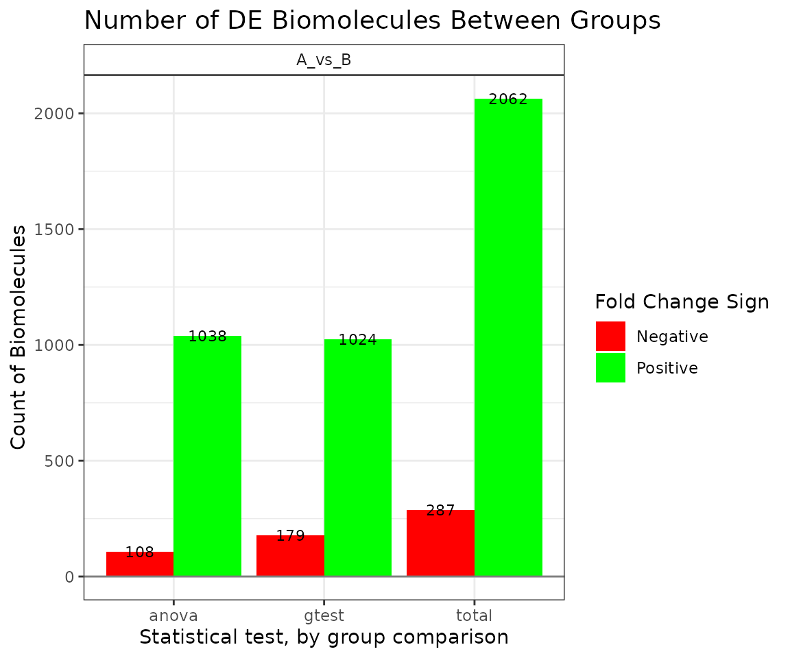

plot(stat_results, plot_type = "volcano")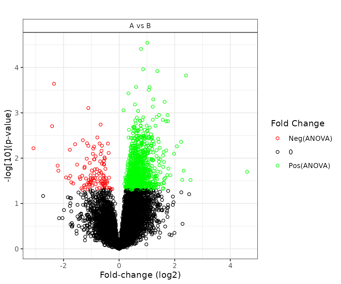

$p$ -value Adjustment Methods

If several comparisons are being made it is a good idea to adjust the $p$ -values in order to control the false positive rate. Currently $p$ -value adjustments are made at the biomolecule level (i.e., adjustments are made for the number of groups being compared). The available $p$ -value adjustments are described in the following table. The “Appropriate Comparison” column refers to which correction method is preferred based on the type of comparisons being made, i.e, all pairwise or case-to-control. Check marks in the “ANOVA” and “IMD” columns indicate if that correction method is appropriate for ANOVA or IMD comparisons.

Method Name	Appropriate Comparison	ANOVA	IMD
Bonferroni	Both	$\sqrt{}$	$\sqrt{}$
Dunnett	Case-vs-control	$\sqrt{}$
Holm	Both	$\sqrt{}$	$\sqrt{}$
Tukey	All pairwise	$\sqrt{}$

False Discovery Rate Methods

To perform false discovery rate (FDR) control, we can pass the argument pval_adjust_a_fdr or pval_adjust_g_fdr for the anova and IMD tests respectively. Options are “bonferroni”, “BH”, “BY”, and “fdr”, see ?p.adjust.

stat_results <- imd_anova(
  omicsData = pep_object,
  test_method = "combined",
  pval_adjust_a_fdr = "BH",
  pval_adjust_g_fdr = "BH"
)

References

Bretz, Frank, Torsten Hothorn, and Peter Westfall. 2016. Multiple Comparisons Using r. CRC Press.

Eddelbuettel, Dirk. 2013. Seamless R and C++ Integration with Rcpp. New York: Springer.

Lenth, Russell V. 2023. Emmeans: Estimated Marginal Means, Aka Least-Squares Means. https://CRAN.R-project.org/package=emmeans.

Webb-Robertson, Bobbie-Jo M, Lee Ann McCue, Katrina M Waters, Melissa M Matzke, Jon M Jacobs, Thomas O Metz, Susan M Varnum, and Joel G Pounds. 2010. “Combined Statistical Analyses of Peptide Intensities and Peptide Occurrences Improves Identification of Significant Peptides from MS-Based Proteomics Data.” Journal of Proteome Research 9 (11): 5748–56.

Bryan Stanfill, Kelly Stratton, Lisa Bramer

2024-10-16

Introduction

IMD-ANOVA Test for Differential Abundance

Analysis of Variance

One Group

Two Groups

Covariate Adjustment

Paired Data

Test for Independence of Missing Data

Covariate Adjustment

Paired Data

Output

Methods for Results Objects

$p$ -value Adjustment Methods

False Discovery Rate Methods

References

Statistical Analysis with the pmartR Package

Bryan Stanfill, Kelly Stratton, Lisa Bramer

2024-10-16

Introduction

IMD-ANOVA Test for Differential Abundance

Analysis of Variance

One Group

Two Groups

Covariate Adjustment

Paired Data

Test for Independence of Missing Data

Covariate Adjustment

Paired Data

Output

Methods for Results Objects

pp-value Adjustment Methods

False Discovery Rate Methods

References

Statistical Analysis with the `pmartR` Package

$p$ -value Adjustment Methods